Problems in Logistic Regression
Today
- Complete and quasi-complete separation
- Log-likelihood with no finite maximizer
- Diagnosing separation
- Separation vs. one extreme observation
- Responses when separation occurs
- Distributional statements and which assumptions transfer
Separation
- Least squares: a formula
\[\widehat\beta = (\mathbf{X}^\top \mathbf{X})^{-1}\mathbf{X}^\top y\]
- Maximum likelihood: \(\widehat\beta\) is the maximizer of \(\ell(\beta)\) — no formula
- A function need not have a maximizer
Perfectly predictive feature
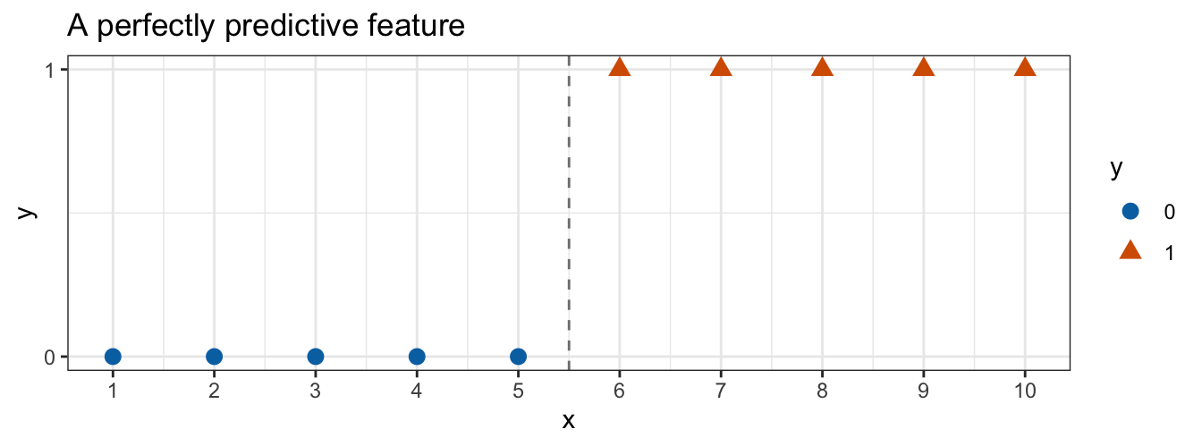
Perfectly predictive feature
Warning: glm.fit: algorithm did not converge
Warning: glm.fit: fitted probabilities numerically 0 or 1 occurred
Call:
glm(formula = y ~ x, family = "binomial", data = toy)

Coefficients:
            Estimate Std. Error z value Pr(>|z|)
(Intercept)   -245.8   337834.2  -0.001    0.999
x               44.7    61172.1   0.001    0.999

(Dispersion parameter for binomial family taken to be 1)

    Null deviance: 1.3863e+01  on 9  degrees of freedom
Residual deviance: 7.8648e-10  on 8  degrees of freedom
AIC: 4

Number of Fisher Scoring iterations: 25
Complete and quasi-complete separation
Complete separation
\[\begin{aligned} x_i b &> 0 \ \text{ for every } i \text{ with } y_i = 1, \\ x_i b &< 0 \ \text{ for every } i \text{ with } y_i = 0 \end{aligned}\]
- \(x_i = (1, x_{i1}, \ldots, x_{ip})\) — feature row for observation \(i\)
- \(b\) — any coefficient vector in \(\mathbb{R}^{p+1}\)
- \(y_i \in \{0, 1\}\) — observed response
- A condition on the data, not on a fitted model
Complete and quasi-complete separation
Quasi-complete separation
\[\begin{aligned} x_i b &\ge 0 \ \text{ for every } i \text{ with } y_i = 1, \\ x_i b &\le 0 \ \text{ for every } i \text{ with } y_i = 0 \end{aligned}\]
- For some \(b \ne 0\), with equality for at least one observation
- Some observations sit exactly on the boundary
- None sits on the wrong side
Tied feature values
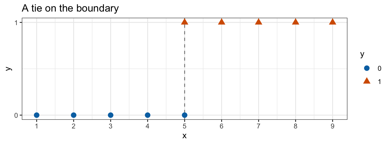
- Two observations at \(x = 5\) with opposite responses
- Dashed line passes through them — no gap left
Tied feature values
\[b = (-5\beta_1, \beta_1), \qquad \beta_1 > 0\]
- \(x = 5\): \(\beta_1(5 - 5) = 0\)
- \(x_i > 5\): \(x_i b > 0\)
- \(x_i < 5\): \(x_i b < 0\)
- Weak inequalities hold for all ten; strict ones fail for two
- Quasi-complete separation
Tied feature values
Warning: glm.fit: fitted probabilities numerically 0 or 1 occurred
Call:
glm(formula = yq ~ xq, family = "binomial", data = quasi)

Coefficients:
            Estimate Std. Error z value Pr(>|z|)
(Intercept)   -98.16   39288.59  -0.002    0.998
xq             19.63    7857.72   0.002    0.998

(Dispersion parameter for binomial family taken to be 1)

    Null deviance: 13.8629  on 9  degrees of freedom
Residual deviance:  2.7726  on 8  degrees of freedom
AIC: 6.7726

Number of Fisher Scoring iterations: 21
Tied feature values
\[\widehat\beta_0 / \widehat\beta_1 = -5\]
- To machine precision
- Iteration walks out along \(b = (-5\beta_1, \beta_1)\), stops at an arbitrary point
Tied feature values
- One warning —
algorithm did not convergedoes not fire - 21 Fisher scoring iterations — short of the default maximum of 25
quasi_glm$converged: TRUE- A reported convergence is not evidence that an estimate is trustworthy
Tied feature values
- Fitted probability at \(x = 5\) stays at \(\text{logistic}(0) = 0.5\)
\[-2\left[\log(0.5) + \log(0.5)\right] = 2.7726\]
- Residual deviance 2.7726, not essentially zero
- Complete separation: deviance falls to zero
- Quasi-complete: deviance falls to what the boundary ties contribute
Maximum likelihood failure
\[\ell(\beta_0, \beta_1) = \sum_{i=1}^n \left\{ y_i (\beta_0 + \beta_1 x_i) - \log\left(1 + e^{\beta_0 + \beta_1 x_i}\right) \right\}\]
- Restrict to \(\beta_0 = -5.5\beta_1\) — boundary fixed at \(x = 5.5\)
- \(\eta_i = \beta_1(x_i - 5.5)\)
Maximum likelihood failure
\[\frac{d\ell}{d\beta_1} = \sum_{i=1}^n (x_i - 5.5)\left(y_i - p_i\right)\]
- \(y_i = 1 \Rightarrow x_i - 5.5 > 0\) and \(y_i - p_i > 0\)
- \(y_i = 0 \Rightarrow x_i - 5.5 < 0\) and \(y_i - p_i < 0\)
- Both cases: positive product
\[\frac{d\ell}{d\beta_1} > 0 \quad \text{for every finite } \beta_1\]
Maximum likelihood failure
- \(\ell < 0\) for every finite \(\beta_1\)
- As \(\beta_1 \to \infty\), \(\ell \to 0\)
- Supremum of \(0\), attained only in the limit
- No finite \(\widehat\beta\) maximizes \(\ell\)
glm()reports wherever the iteration stopped; SEs grow as the curvature flattens
Maximum likelihood failure
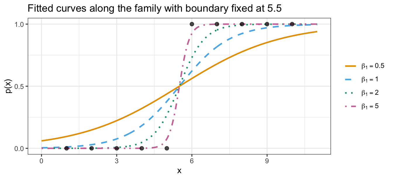
Maximum likelihood failure
| \(\beta_1\) | \(\ell(\beta_1)\) | \(L(\beta_1)\) |
|---|---|---|
| 0.0 | -6.931 | 0.001 |
| 0.5 | -2.950 | 0.052 |
| 1.0 | -1.590 | 0.204 |
| 2.0 | -0.739 | 0.477 |
| 5.0 | -0.159 | 0.853 |
| 8.0 | -0.036 | 0.964 |
Maximum likelihood failure
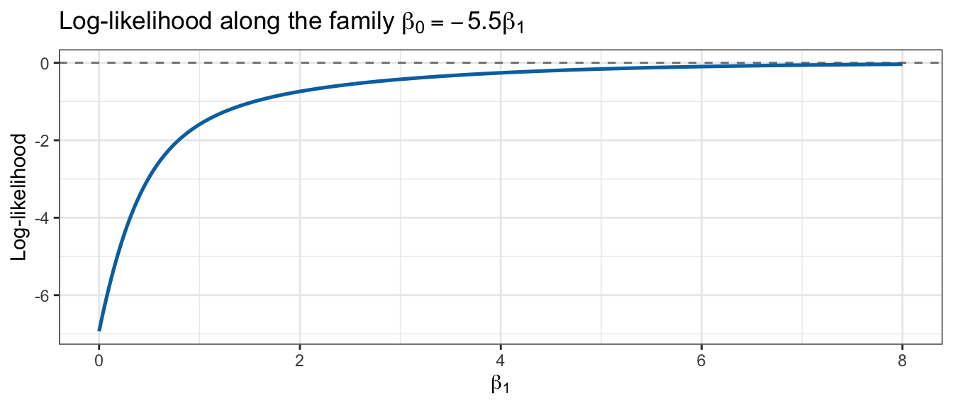
Muscular dystrophy carrier screening
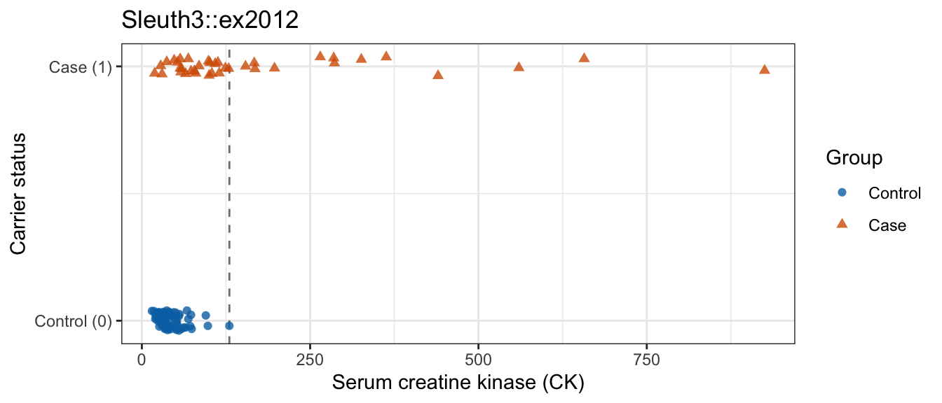
Sleuth3::ex2012— carrier status vs. serum creatine kinase (CK)- Groups overlap heavily below the dashed line
- Not separated under either definition
Muscular dystrophy carrier screening
Warning: glm.fit: fitted probabilities numerically 0 or 1 occurred Estimate Std. Error z value Pr(>|z|)
(Intercept) -3.96219273 0.6719084 -5.896924 3.703413e-09
CK 0.05073407 0.0106958 4.743364 2.101984e-06- Same warning as the toy example — different reason (
converged: TRUE, 7 iterations)
Muscular dystrophy carrier screening
| CK | Group | \(\widehat\eta\) | \(1 - \widehat p\) |
|---|---|---|---|
| 925 | Case | 43.0 | \(2.2 \times 10^{-16}\) |
| 657 | Case | 29.4 | \(1.8 \times 10^{-13}\) |
| 560 | Case | 24.4 | \(2.4 \times 10^{-11}\) |
| 440 | Case | 18.4 | \(1.1 \times 10^{-8}\) |
| 363 | Case | 14.5 | \(5.3 \times 10^{-7}\) |
Muscular dystrophy carrier screening
\[1 - \text{logistic}(\widehat\eta) = \frac{e^{-\widehat\eta}}{1 + e^{-\widehat\eta}}\]
- One woman’s \(\widehat\eta = 42.97 \Rightarrow\) true gap \(2.2 \times 10^{-19}\)
- No double holds a probability that close to 1
glm()clamps the linear predictor before inverting the linkfitted()never leaves \([2.2 \times 10^{-16},\ 1 - 2.2 \times 10^{-16}]\)
Muscular dystrophy carrier screening
- Each \(+10\) units of
CK\(\times\ 1.66\) odds of carrier (95% CI 1.35–2.05) - Estimate finite, SE small relative to it, converged
- Warning here: one extreme observation, not a failed estimator
Recognizing separation
glm.fit: algorithm did not converge— close to conclusiveglm.fit: fitted probabilities numerically 0 or 1 occurred— not conclusive alone; separation always produces it
Recognizing separation
- A coefficient absurd on the feature’s own scale — odds ratio \(e^{44.7}\) per unit
- SE far larger than the coefficient: \(z \approx 0\), \(p\)-value near 1
- Residual deviance essentially zero (complete) or small (quasi-complete)
fitted()numerically 0 or 1 on the separated side
Recognizing separation
- Compare \(|\widehat\beta_j|\) against its SE — one line, settles the question
fit$converged— informative only whenFALSE- Quasi-complete separation can report convergence and still leave no usable estimate
Available responses
- Collect more data — separation is a property of a sample, not of the population
- Simplify the model — drop or merge the feature or level causing it
- Use the fit for what it can still support — separation destroys the coefficient, not necessarily the classification
Linear regression problems revisited
Six potential problems from the flexibility lecture:
- Non-linearity, correlated errors, non-constant variance
- Outliers, high-leverage points, collinearity
Separation: no counterpart — least squares evaluates a formula
Linear regression problems revisited
\[Y_i \mid x_i \stackrel{ind}{\sim} N\left(x_i\beta, \sigma^2\right), \qquad i = 1, \ldots, n\]
- \(Y_i\) — response for observation \(i\)
- \(x_i = (1, x_{i1}, \ldots, x_{ip})\) — \(i\)th row of \(\mathbf{X}\)
- \(\beta = (\beta_0, \beta_1, \ldots, \beta_p)^\top\) — coefficient vector; \(x_i\beta\) — linear predictor
- \(\sigma^2\) — variance around the linear predictor
Linear regression problems revisited
Four assumptions in one line:
- Independence — the \(\mathrm{ind}\) over the \(\sim\)
- Constant variance — \(Var[Y_i \mid x_i] = \sigma^2\), no \(i\) subscript
- Linearity — \(E[Y_i \mid x_i] = x_i\beta\)
- Normality — normally distributed around its mean
Linear regression problems revisited
\[Y_i \mid x_i \stackrel{ind}{\sim} \text{Bernoulli}\left(p(x_i)\right), \qquad \log\left[\frac{p(x_i)}{1 - p(x_i)}\right] = x_i\beta\]
- \(p(x_i) = P(Y_i = 1 \mid x_i)\) — probability of the event for observation \(i\)
- Normal \(\to\) Bernoulli; identity link \(\to\) logit
Linear regression problems revisited
Four assumptions after the substitution:
- Independence — still assumed; can still fail
- Constant variance — not assumed; \(Var[Y_i \mid x_i] = p(x_i)[1 - p(x_i)]\) follows from the Bernoulli
- Linearity — still assumed, of the log-odds
- Normality — gone, replaced by the Bernoulli
Independence
- Bernoulli log-likelihood is a sum over observations — because they were assumed independent
- No \(\epsilon_i\): correlated observations, not correlated errors
- Positively correlated observations carry less information than their count suggests
- Every standard error from
glm()too small
Independence
- Time — a patient at successive visits, a stock’s daily direction
- Space — counties, plots in a field, weather stations
- Clustering — students within schools, patients within hospitals, repeated measurements on the same subject
Independence
Add features that explain the source of the correlation
- A cluster-identifying factor
- A time index or trend
- The spatial coordinates
- Responses independent given the features
Variance
- Linear regression: \(Var[Y_i \mid x_i] = \sigma^2\) — assumed; check for a fan shape in residuals vs. fitted
- Logistic regression:
\[Var[Y_i \mid x_i] = p(x_i)\left[1 - p(x_i)\right]\]
- A consequence of Bernoulli, not an extra assumption; no \(\sigma^2\)
- A residual plot that fans out is not evidence against the model
Variance
Aggregated data: \(m_i\) trials per row
\[Y_i \mid x_i \stackrel{ind}{\sim} \text{Binomial}(m_i, p(x_i))\]
- Variance \(m_i p(x_i)[1 - p(x_i)]\)
- Overdispersion — spread of the \(Y_i\) around their fitted means exceeds that
Variance
Overdispersion: usually a symptom of failed independence
- Positively correlated trials within a row — same school, same clutch of eggs, same subject
- Adds covariance terms independence would have set to zero
- Unmodeled features that vary within a row: same excess
Linearity
\[\log\left[\frac{p(x_i)}{1 - p(x_i)}\right] = x_i\beta\]
- Can fail
- Interactions — a feature’s log-odds slope depends on another feature
- Polynomial and step-function columns — bend within a single feature
- Fit the more flexible model, test the added coefficients
Collinearity, leverage, and outliers
- Carry over in substance
- Collinearity: \(\text{SE}(\widehat\beta_j)\) inflates, \(z\)-test loses power
- Unusual feature value: still disproportionate pull
- Disagreeing response: still distorts the fit
- Arithmetic does not carry over: \(H = \mathbf{X}(\mathbf{X}^\top \mathbf{X})^{-1}\mathbf{X}^\top\), studentized residuals, Cook’s distance
Conclusion
- Complete and quasi-complete separation
- Supremum without a finite maximizer
- Separation signature
- Coefficient table, not the warning
- Distributional statements
- Independence: time, space, clustering
- Overdispersion
- Collinearity, leverage, outliers: concepts, not formulas
DS 3030