Principal Components
Today
- Diamond measurements
- First principal component
- Loadings and scores
- Maximum variance
- Closest line
- Later components
- Orthogonal directions
- Variance explained
- Components kept
- Scaling
- Interpretation
- Loadings
- Unsupervised learning
Diamond measurements
- Question: can fewer than six directions capture most of the variation in these numbers?
- Explanatory variables:
carat,depth,table,x,y,z
- Features: these six, standardized
- Response variable:
price, not used in this lecture
Correlated measurements
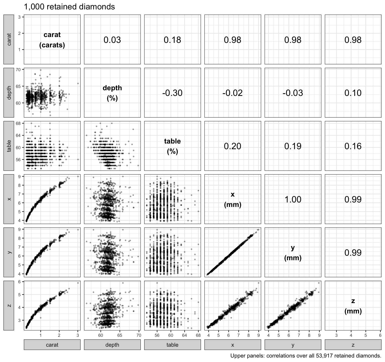
Features
\[\tilde x_{ij} = \frac{x_{ij} - \bar x_j}{s_j}, \qquad s_j = \sqrt{\frac{1}{n}\sum_{i=1}^n\left(x_{ij} - \bar x_j\right)^2}\]
- \(x_{ij}\) — explanatory variable \(j\) of diamond \(i\)
- \(\bar x_j\), \(s_j\) — mean and standard deviation of explanatory variable \(j\)
- \(\tilde x_{ij}\) — feature \(j\) of diamond \(i\)
\[\mathbf{R} = \frac{1}{n}\tilde{\mathbf{X}}^\top\tilde{\mathbf{X}}\]
- \(\mathbf{R}\) — sample correlation matrix
First principal component
Two features
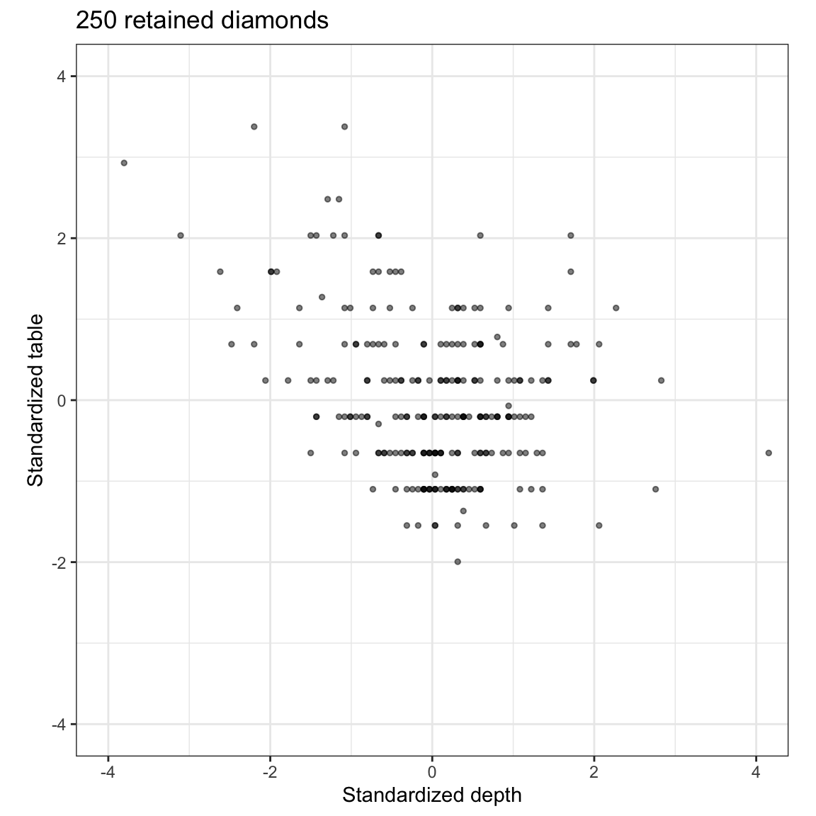
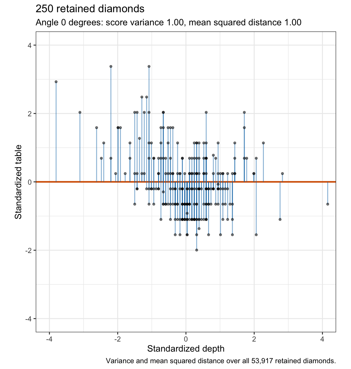
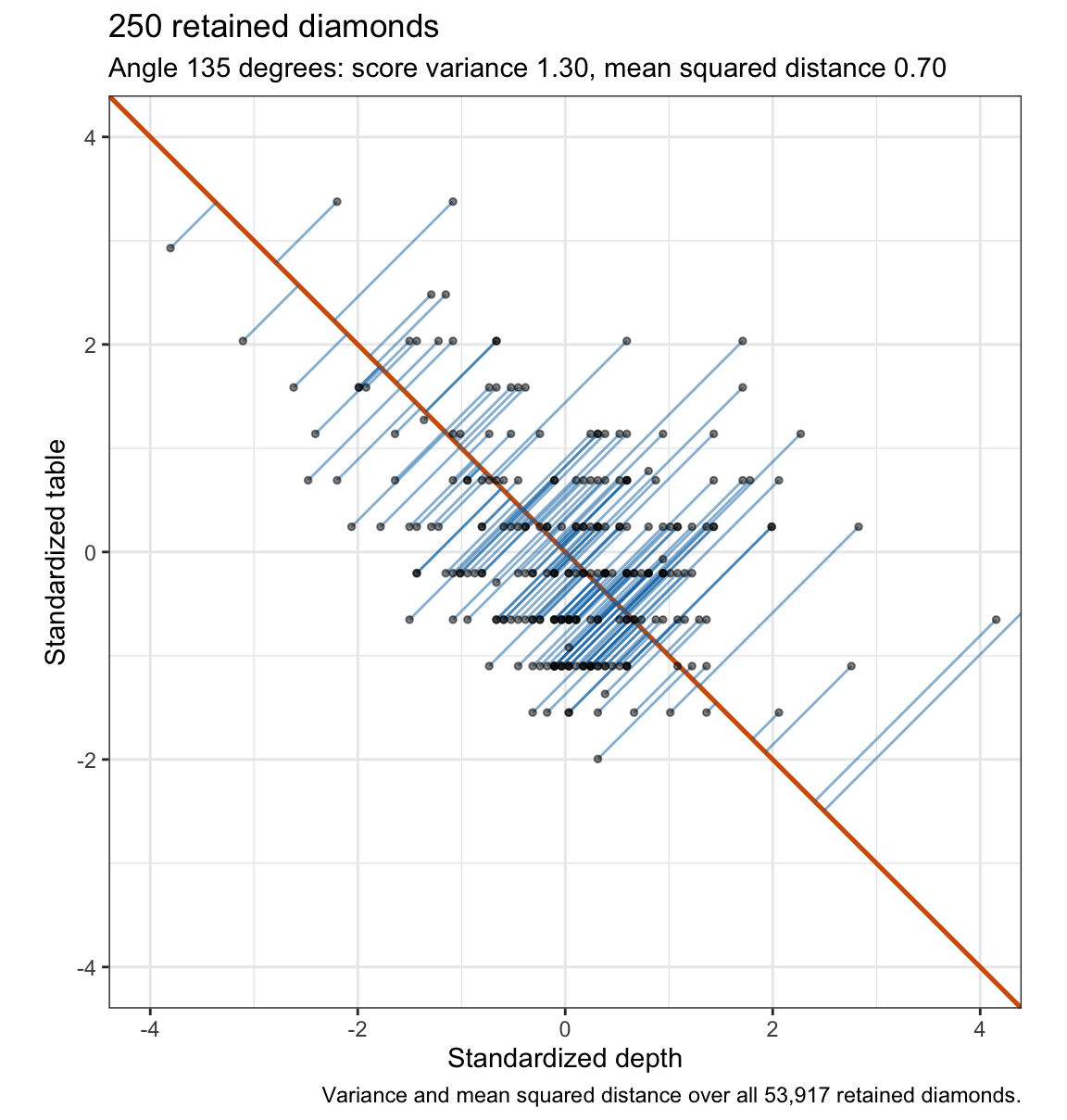
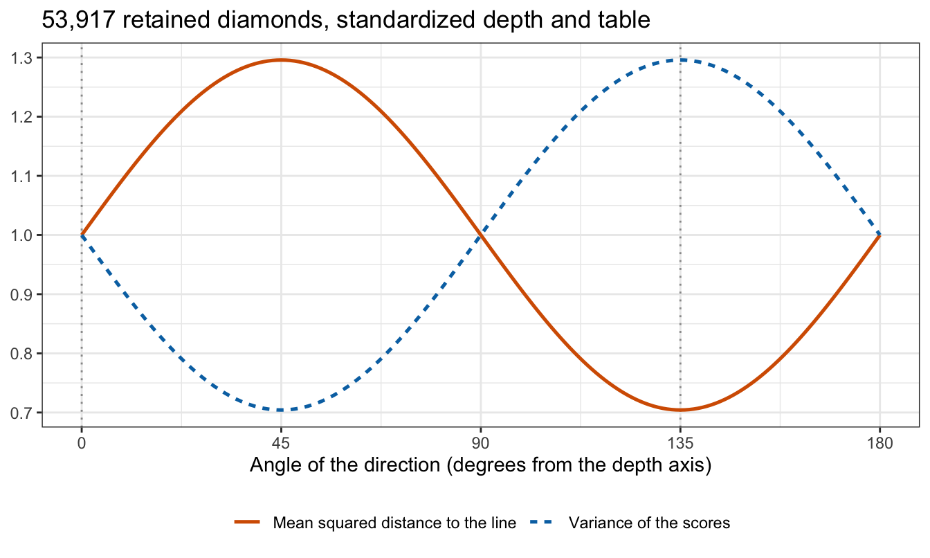
Loadings and scores
\[Z_1 = \phi_{11}\tilde X_1 + \phi_{21}\tilde X_2 + \cdots + \phi_{p1}\tilde X_p, \qquad \sum_{j=1}^p\phi_{j1}^2 = 1\]
- \(Z_1\) — first principal component: the combination with the largest sample variance
- \(\tilde X_j\) — feature \(j\)
- \(\phi_{j1}\) — loading of feature \(j\); \(\phi_1 = \left(\phi_{11}, \ldots, \phi_{p1}\right)^\top\) — loading vector
\[z_{i1} = \sum_{j=1}^p\phi_{j1}\tilde x_{ij} = \tilde x_i\phi_1\]
- \(z_{i1}\) — score of diamond \(i\)
Maximum variance
Sample variance of the scores of a unit vector \(a\)
\[\frac{1}{n}\sum_{i=1}^n\left(\tilde x_i a\right)^2 = \frac{1}{n}a^\top\tilde{\mathbf{X}}^\top\tilde{\mathbf{X}}a = a^\top\mathbf{R}a\]
Maximize \(a^\top\mathbf{R}a\) subject to \(a^\top a = 1\)
\[2\mathbf{R}a - 2va = 0 \quad\Rightarrow\quad \mathbf{R}a = va\]
- \(v\) — Lagrange multiplier
- \(\phi_1\) — eigenvector of \(\mathbf{R}\) with the largest eigenvalue \(v_1\)
- \(v_1\) — variance of the first component’s scores
Closest line
\[\left\|\tilde x_i\right\|^2 = z_{i1}^2 + \left\|\tilde x_i - z_{i1}\phi_1^\top\right\|^2\]
\[\frac{1}{n}\sum_{i=1}^n\left\|\tilde x_i - z_{i1}\phi_1^\top\right\|^2 = p - \phi_1^\top\mathbf{R}\phi_1\]
- \(\left\|\tilde x_i - z_{i1}\phi_1^\top\right\|^2\) — squared distance from diamond \(i\) to the line
- \(\phi_1^\top\mathbf{R}\phi_1\) — variance of the scores
Later components
Orthogonal directions
\(m\)th component: maximum variance among unit vectors orthogonal to \(\phi_1, \ldots, \phi_{m-1}\)
\[v_1 \ge v_2 \ge \cdots \ge v_p \ge 0\]
- \(\phi_m\) — eigenvector of \(\mathbf{R}\) with the \(m\)th largest eigenvalue \(v_m\)
- \(v_m\) — variance of the \(m\)th component’s scores
- scores of different components are uncorrelated
\[\sum_{m=1}^p v_m = \operatorname{tr}\left(\mathbf{R}\right) = p\]
- \(p\) — total variance of the standardized features
Variance explained
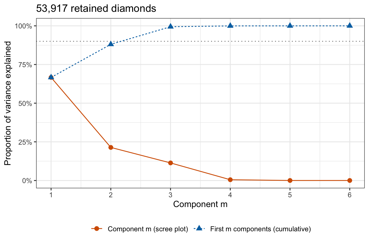
\[\text{PVE}_m = \frac{v_m}{\sum_{l=1}^p v_l} = \frac{v_m}{p}\]
- \(v_m\) — variance of the \(m\)th component’s scores
- \(p\) — total variance of the standardized features
- \(\sum_{m=1}^M\text{PVE}_m\) — cumulative PVE of the first \(M\) components
Variance explained by component
| Component | Variance \(v_m\) | PVE | Cumulative PVE |
|---|---|---|---|
| PC1 | 3.999 | 66.66% | 66.66% |
| PC2 | 1.284 | 21.40% | 88.06% |
| PC3 | 0.683 | 11.38% | 99.44% |
| PC4 | 0.031 | 0.52% | 99.95% |
| PC5 | 0.002 | 0.03% | 99.98% |
| PC6 | 0.001 | 0.02% | 100.00% |
Scree plot
Components kept
- Elbow: keep the components before the scree plot flattens
- Cumulative threshold: keep the fewest components whose cumulative PVE reaches a chosen level
- Diamonds: \(M = 3\) by both rules
- Both are judgments
Scaling
Raw units
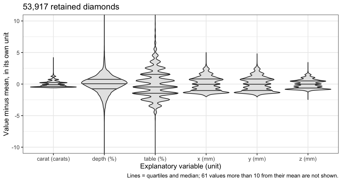
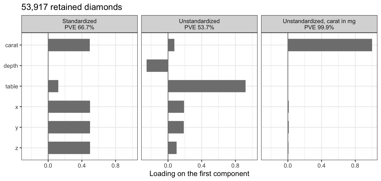
Unstandardized components
Interpretation
Loadings
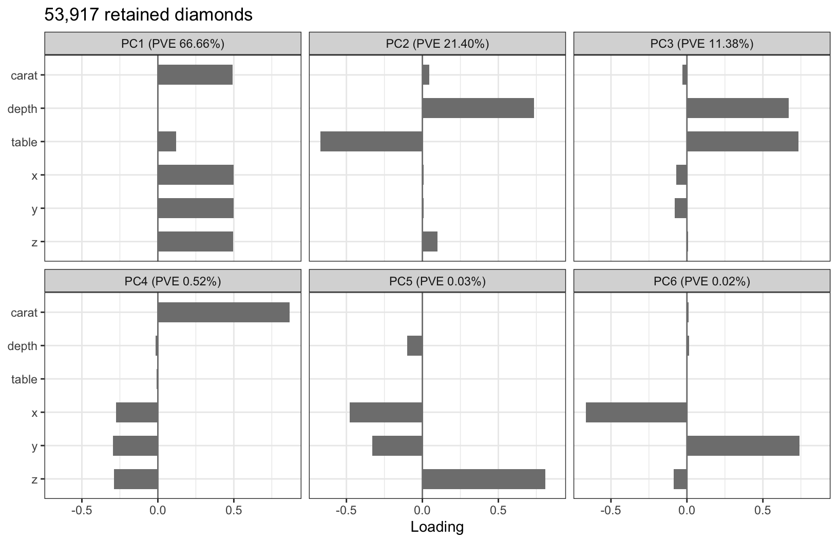
Reading the loadings
- PC1, size: high score is a large diamond
- PC2, depth against table: high score is deep with a narrow table
- PC3, depth and table together: high score is deep and wide-topped
- PC4 to PC6, disagreements among the size measures
- The sign of a loading vector is arbitrary
Scores
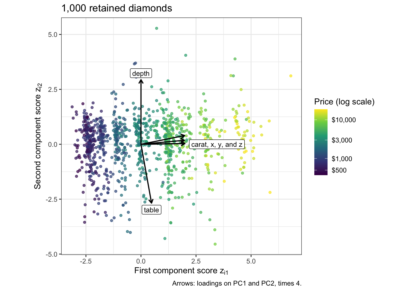
Price
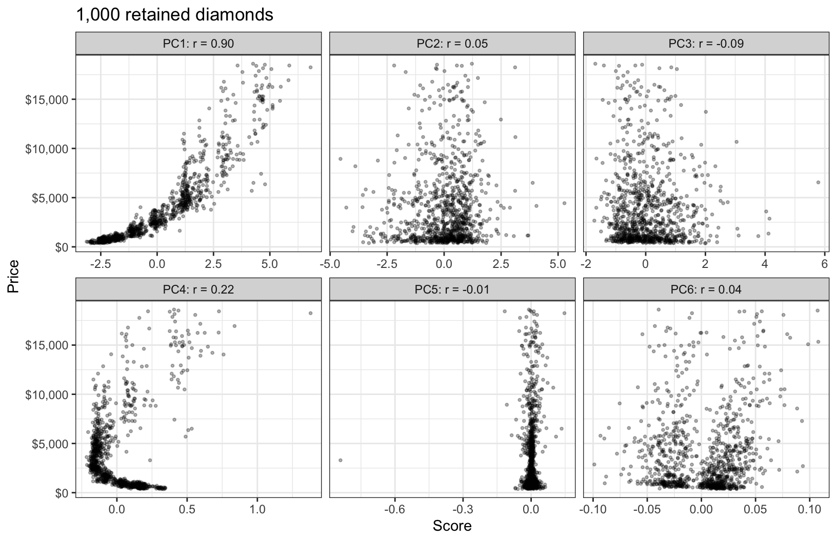
Prediction
- Unsupervised: computed from the features alone
- The component with the most variance need not be the best predictor
- Not variable selection: every component uses all \(p\) features
Conclusion
- Components are directions of decreasing variance of the features
- The first component is the top eigenvector and the closest line
- Choose \(M\) from the scree plot or a cumulative PVE; both are judgments
- Standardize the features unless the units are comparable
- Components ignore the response and use every feature
DS 3030