High Dimensions
Today
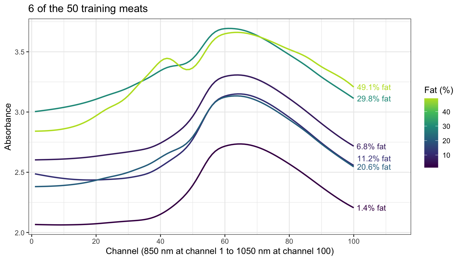
- Meat spectra
- Data
- Least squares
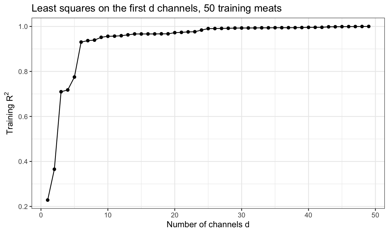
- Perfect fits
- Channel sweep
- Inference
- Penalized criteria
- AIC
- Regularization
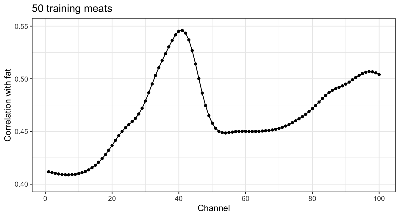
- Channels and fat
- Four methods
- Computation
- Tuning
- Test MSE
- Selected channels
Meat spectra
- Question: from a small training sample, how well can the fat content of chopped meat be predicted from its absorbance at each of 100 channels?
- Observation: a meat, a sample of finely chopped meat
- Response variable:
fat, in percent - Explanatory variables: absorbance at 100 channels,
x_001, …,x_100
- Training sample: 50 meats, so \(p = 100 > n = 50\)
- Test meats: 143
Data
Least squares
Perfect fits
\[\mathbf{X}^\top\mathbf{X}\,b = \mathbf{X}^\top y\]
- \(\mathbf{X}\) — \(n \times (p + 1)\) model matrix, a column of ones and one column per channel
- \(b\) — \((p + 1)\)-vector of candidate estimates, the intercept first
- \(y\) — \(n\)-vector of the training responses
- \(p + 1 > n\): \(\mathbf{X}^\top\mathbf{X}\) is singular, so the estimate is not unique
- Rank \(n\): the fitted values equal the responses, training RSS 0 and training \(R^2 = 1\)
- \(RSS = \sum_{i=1}^n\left(y_i - \widehat y_i\right)^2\) — training residual sum of squares
Channel sweep
Inference
\[H_0: \beta_1 = \cdots = \beta_d = 0\]
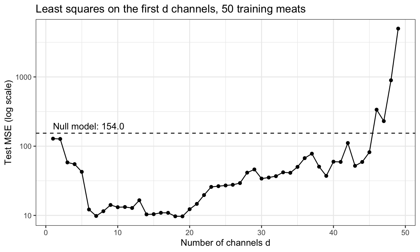
- \(d = 46\): overall \(F\)-test \(p\)-value 0.0016, training \(R^2\) 0.9993
- None of the 46 estimates has a \(p\)-value below 0.05
- \(\widehat\sigma = 1.49\) percentage points, but the test root mean squared error is 18.3
Penalized criteria
\[C_p = \frac{1}{n}\left(RSS + 2d\widehat\sigma^2\right), \qquad \text{BIC} = \frac{1}{n}\left[RSS + \log(n)\,d\widehat\sigma^2\right]\]
- \(\sigma^2\) fixed at \(\widehat\sigma^2\) from the model with all \(p\) features: its \(RSS\) over \(n - \text{rank}(\mathbf{X})\)
- \(\text{rank}(\mathbf{X}) = n\): \(\widehat\sigma^2 = 0/0\), undefined
- \(\widehat\sigma^2 = 0\): \(C_p\) and BIC reduce to \(RSS/n\), smallest for the largest model
AIC
- Subset selection lecture’s AIC: \(\sigma^2\) fixed at \(\widehat\sigma^2\), equivalent to \(C_p\)
AIC()andBIC()in R: \(\sigma^2\) estimated in each model by \(RSS/n\)
\[-2\log L = n\log\left(2\pi\,RSS/n\right) + n\]
- As \(RSS \to 0\), \(-2\log L \to -\infty\): both smallest at \(d = 49\), where they are \(-\infty\)
Regularization
Channels and fat
Four methods
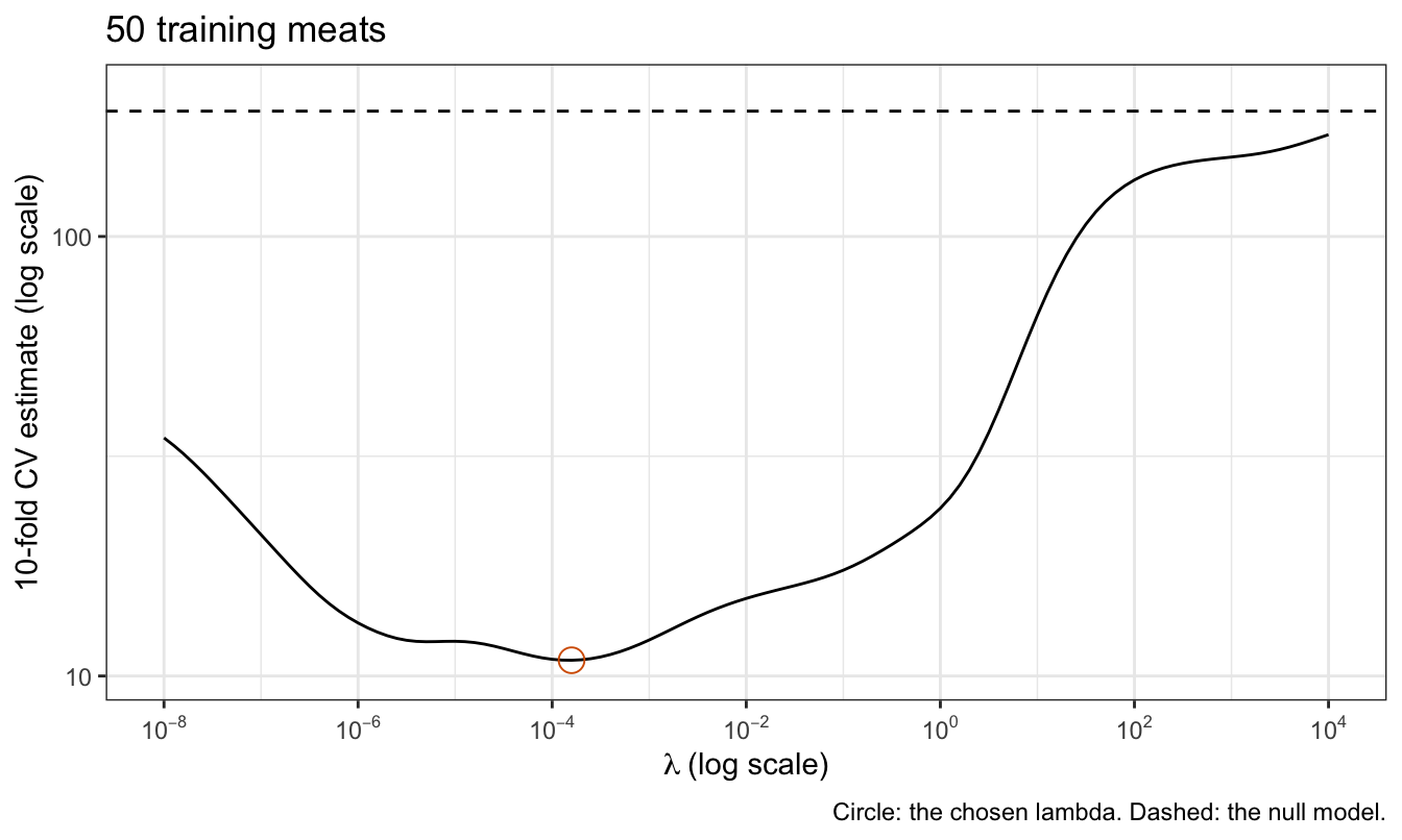
- Ridge regression: minimize \(RSS + \lambda\sum_{j=1}^p\beta_j^2\)
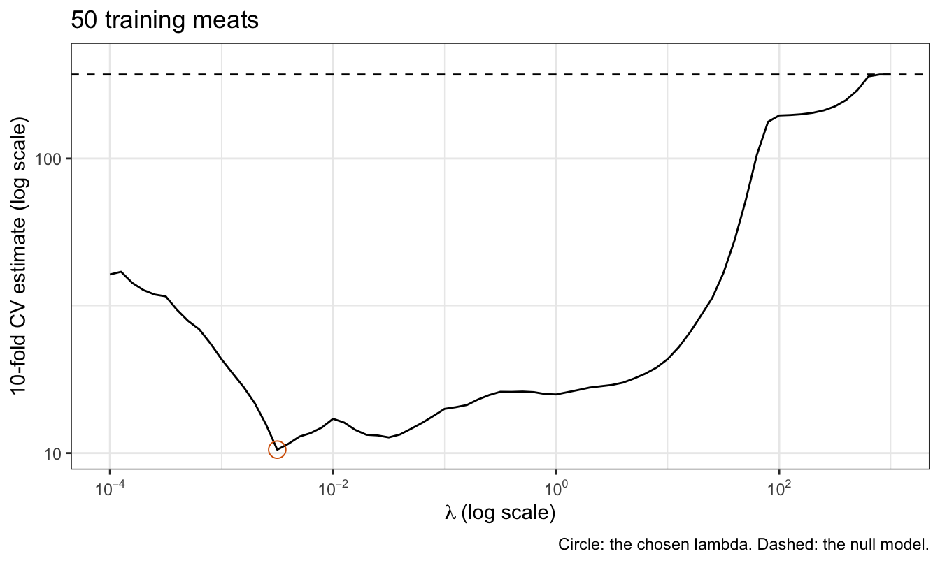
- Lasso: minimize \(RSS + \lambda\sum_{j=1}^p\left|\beta_j\right|\)
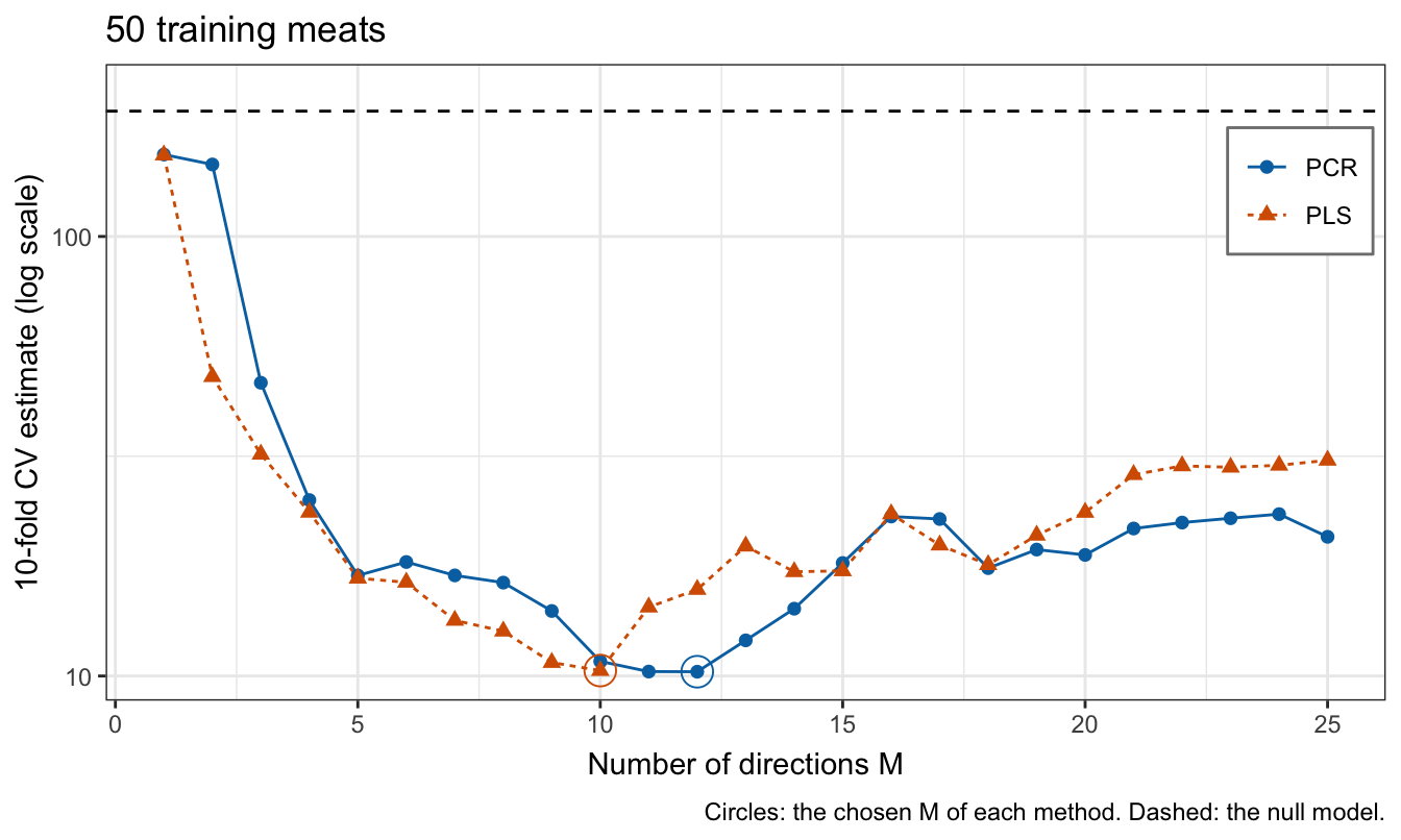
- PCR: regress fat on the first \(M\) principal component scores
- PLS: regress fat on \(M\) directions chosen with the response
- \(\lambda \ge 0\) — tuning parameter
- \(\lambda\) or \(M\) chosen by 10-fold cross-validation
- Standardization, components and directions recomputed in each fold
Computation
\[\widehat\beta^R_\lambda = \left(\tilde{\mathbf{X}}^\top\tilde{\mathbf{X}} + \lambda\mathbf{I}_p\right)^{-1}\tilde{\mathbf{X}}^\top\left(y - \bar y\mathbf{1}\right)\]
- \(\mathbf{I}_p\) — \(p \times p\) identity matrix
- \(\bar y\) — mean of the training responses \(y\); \(\mathbf{1}\) — \(n\)-vector of ones
\[\tilde{\mathbf{x}}_{\cdot j}^\top r = \frac{\lambda}{2}\,\text{sign}\left(\widehat\beta^L_{\lambda j}\right) \quad \text{if } \widehat\beta^L_{\lambda j} \ne 0, \qquad \left|\tilde{\mathbf{x}}_{\cdot j}^\top r\right| \le \frac{\lambda}{2} \quad \text{if } \widehat\beta^L_{\lambda j} = 0\]
- \(r = y - \bar y\mathbf{1} - \tilde{\mathbf{X}}\widehat\beta^L_\lambda\) — residuals
- \(\tilde{\mathbf{x}}_{\cdot j}\) — column \(j\) of \(\tilde{\mathbf{X}}\)
Tuning
Test MSE
| Method | Tuning | Nonzero | 10-fold CV | Test MSE |
|---|---|---|---|---|
| Null | 0 | 192.81 | 153.95 | |
| Ridge | \(\lambda = 1.6 \times 10^{-4}\) | 100 | 10.86 | 8.09 |
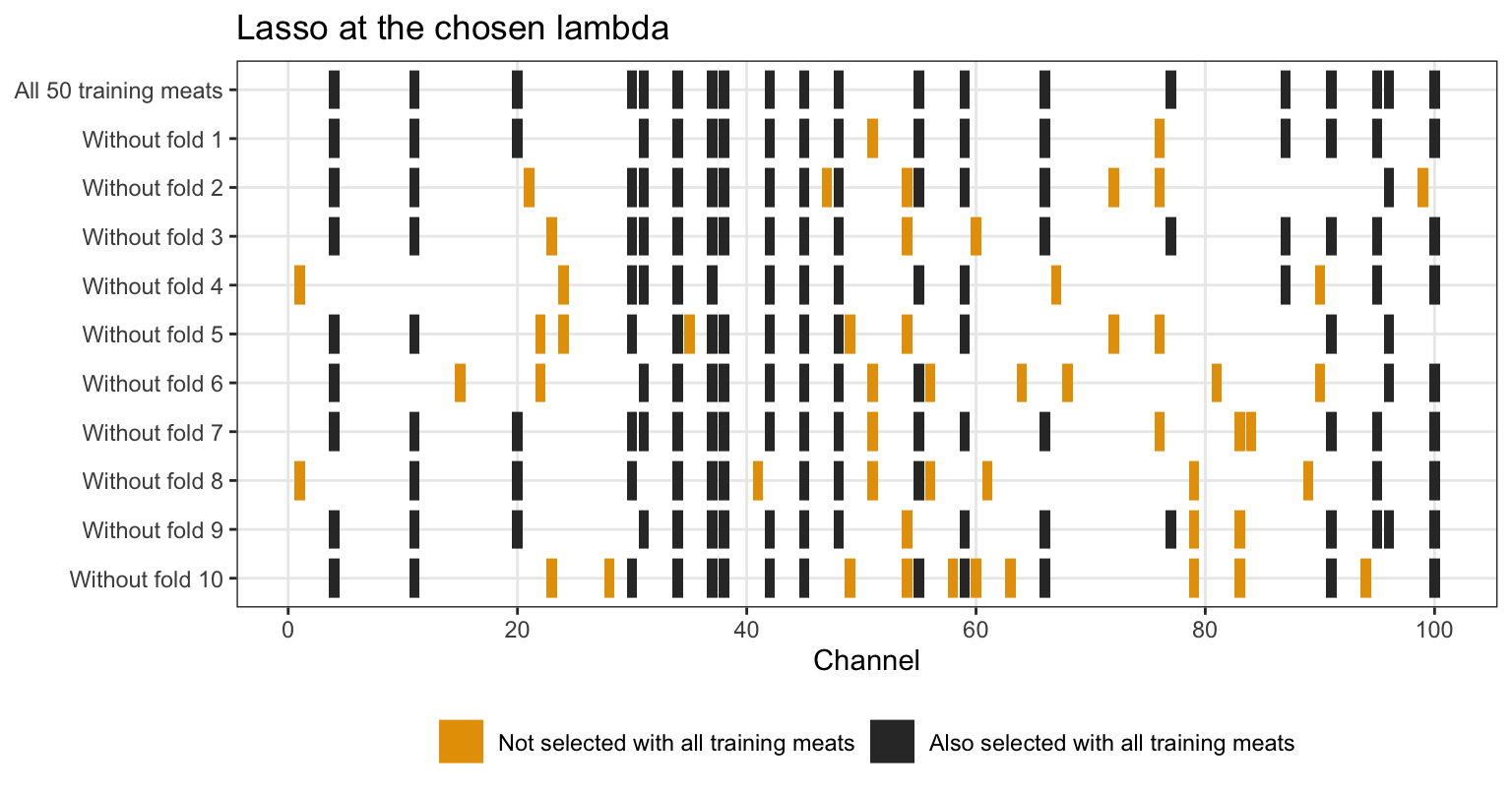
| Lasso | \(\lambda = 3.2 \times 10^{-3}\) | 20 | 10.27 | 13.26 |
| PCR | \(M = 12\) | 100 | 10.23 | 8.71 |
| PLS | \(M = 10\) | 100 | 10.29 | 9.52 |
Selected channels
Conclusion
- Least squares fails when \(p + 1 > n\)
- Training \(R^2\) and training MSE cannot choose among fits
- \(C_p\), BIC and AIC with fixed \(\sigma^2\) need an estimate that is \(0/0\)
AIC()andBIC()go to \(-\infty\) at a perfect fit- Cross-validate \(\lambda\) or \(M\), recomputing every step in each fold
- Correlated features: the lasso’s set changes from fold to fold
DS 3030