Decision Trees
Today
- Concrete strength
- Data
- Training specimens
- Regression trees
- Regions and predictions
- Best split
- Recursive binary splitting
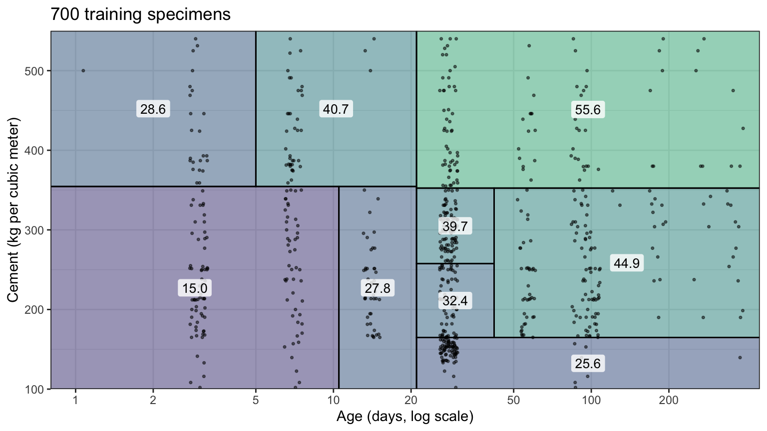
- Fitting and partition
- Pruning
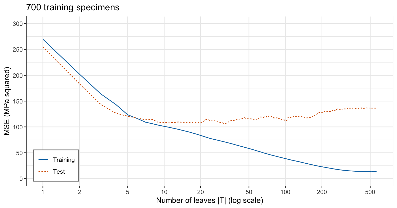
- Overfitting
- Cost-complexity pruning
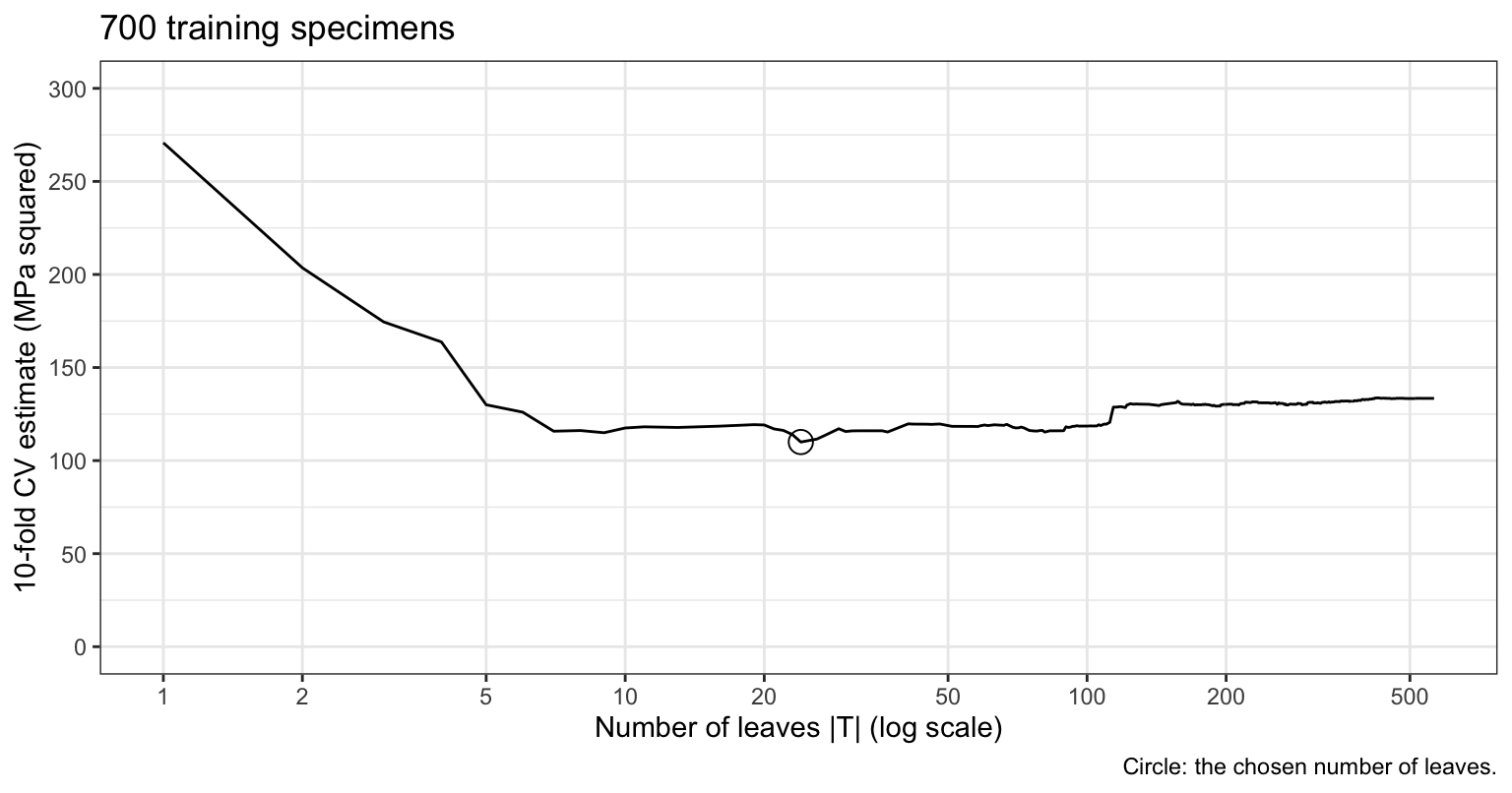
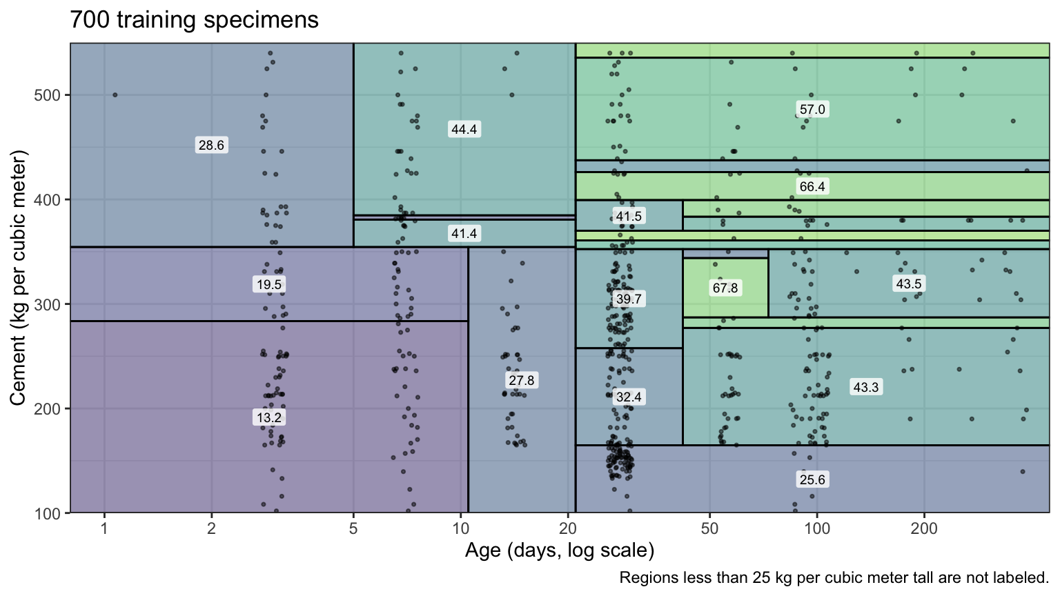
- Cross-validation and pruned tree
- All explanatory variables
- Classification trees
- Penguin species
- Most common class
- Node impurity
- Fitting and pruning
- Strengths and weaknesses
- Interpretability and nonlinearity
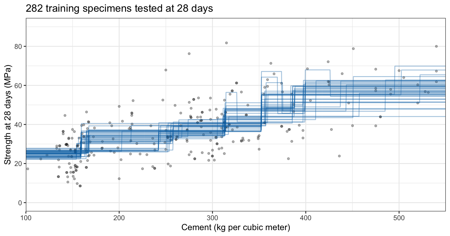
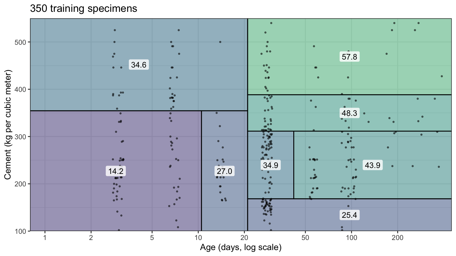
- Step functions and instability
Concrete strength
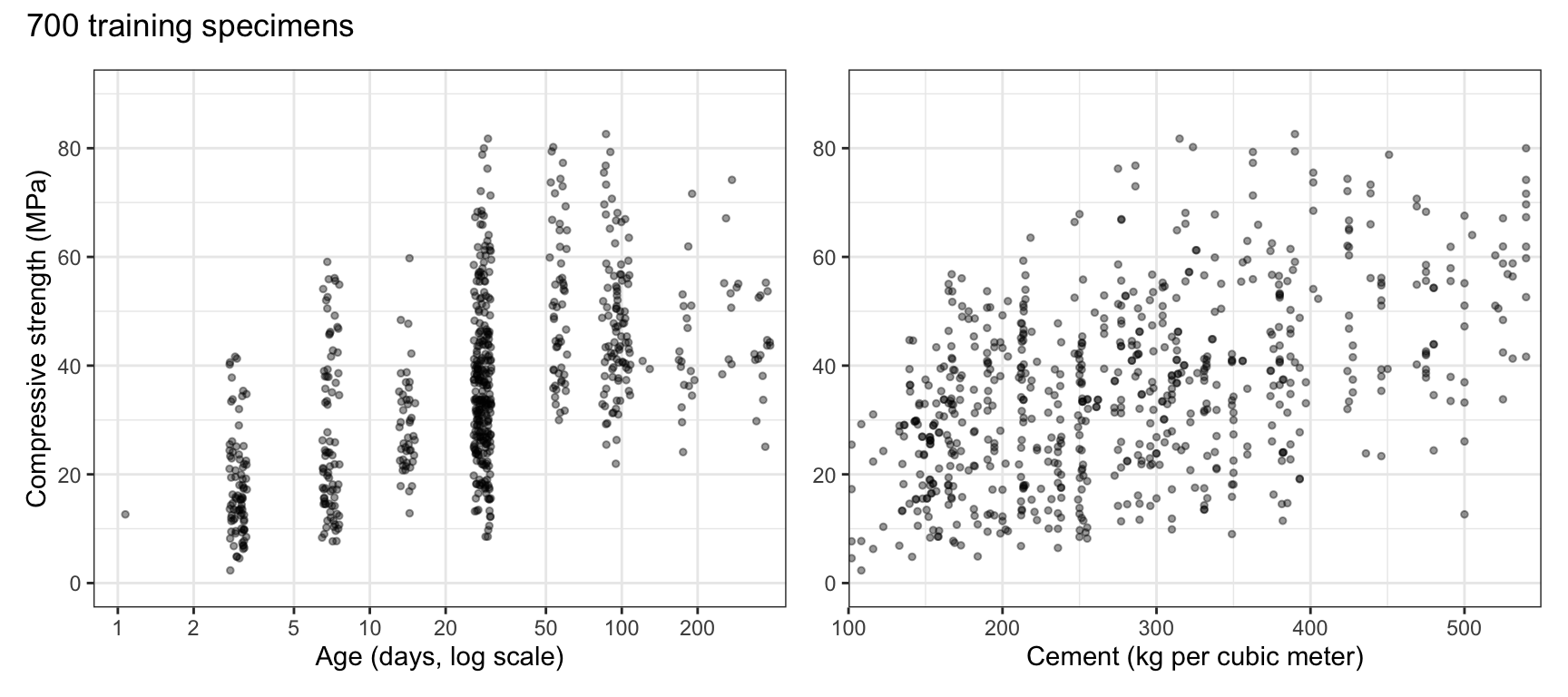
Data
- Question: how well do the ingredients of a concrete mix and its age predict how much load the concrete can bear?
- Observation: a specimen, one cylinder of one mix, crushed at one age
- Response variable:
compressive_strength, in megapascals (MPa) - Explanatory variables: seven ingredients, in kg per cubic meter of mix, and
age, in days
- Training sample: 700 specimens
- Test specimens: 305
Training specimens
Regression trees
Age and cement
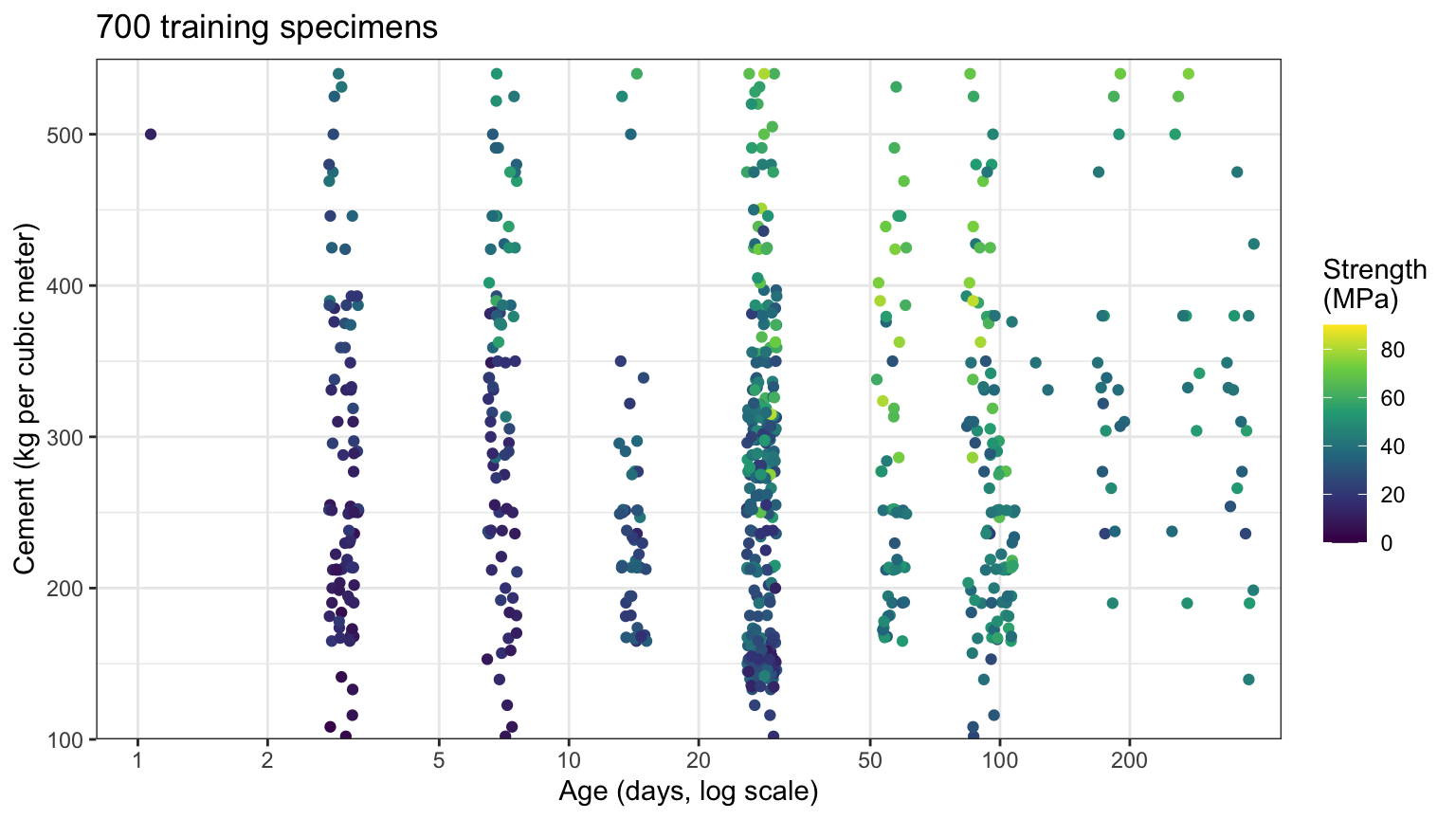
Regions and predictions
\[\widehat f(x) = \sum_{\ell=1}^{L} \widehat y_{R_\ell}\,\mathrm{I}\left(x \in R_\ell\right),\]
- \(x\) — value of the \(p\) explanatory variables \(X = (X_1, \ldots, X_p)\)
- \(R_\ell\) — \(\ell\)th region, a rectangle in the \(p\) explanatory variables
- \(\widehat y_{R_\ell}\) — mean response of the training observations in \(R_\ell\)
- \(\mathrm{I}\left(x \in R_\ell\right)\) — 1 if \(x\) falls in \(R_\ell\), 0 otherwise
\[\text{RSS} = \sum_{\ell=1}^{L}\sum_{i:\, x_i \in R_\ell}\left(y_i - \widehat y_{R_\ell}\right)^2.\]
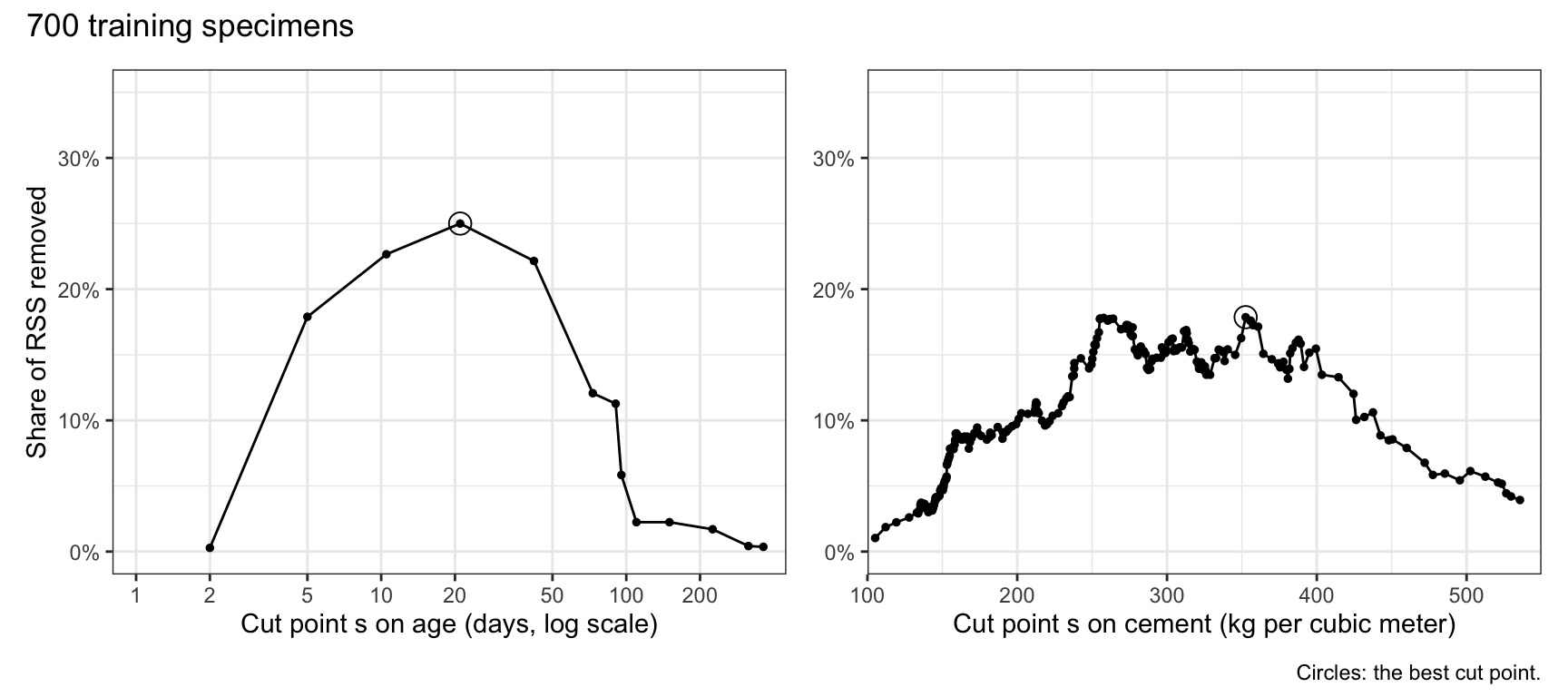
Best split
\[R_1(j, s) = \left\{X \in R \mid X_j < s\right\}, \qquad R_2(j, s) = \left\{X \in R \mid X_j \ge s\right\}\]
- \(R\) — region being split
- \(X_j\) — explanatory variable \(j\)
- \(s\) — cut point
\[\sum_{i:\, x_i \in R_1(j, s)}\left(y_i - \widehat y_{R_1}\right)^2 + \sum_{i:\, x_i \in R_2(j, s)}\left(y_i - \widehat y_{R_2}\right)^2\]
- RSS of the two regions after the split, minimized over \((j, s)\)
Decrease in RSS
- RSS before the split minus RSS after it
\[n_1\left(\bar y_1 - \bar y\right)^2 + n_2\left(\bar y_2 - \bar y\right)^2 = \frac{n_1 n_2}{n_1 + n_2}\left(\bar y_1 - \bar y_2\right)^2.\]
- \(n_1, n_2\) — training observations in the two regions
- \(\bar y_1, \bar y_2\) — their means
- \(\bar y\) — mean before the split
Best split: cut points
Recursive binary splitting
- Start with all the training observations in one region, the root
- In each current region, find the best split \((j, s)\) of the training observations in that region alone, and split
- Repeat in each new region until a stopping rule holds
- Greedy: each split is the best one at its own step
- Top-down: from the root to the leaves
- Default stopping rules: fewer than 20 observations in a region, a leaf with fewer than 7, a split lowering the RSS by less than 1% of the root’s
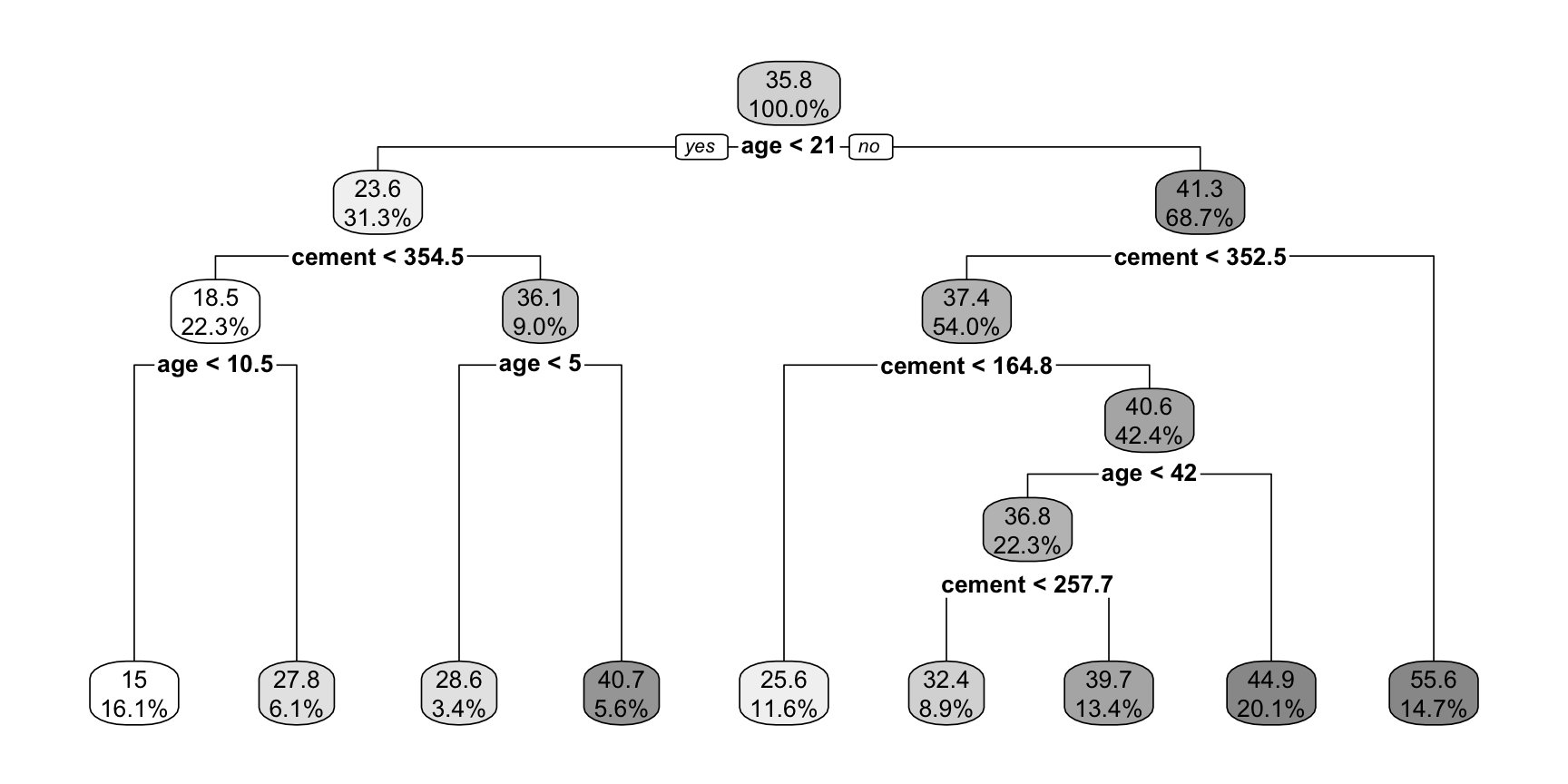
Fitting a regression tree
n= 700

node), split, n, deviance, yval
      * denotes terminal node

 1) root 700 188853.400 35.76574
   2) age< 21 219  35098.050 23.59484
     4) cement< 354.5 156  11805.220 18.54385
       8) age< 10.5 113   4471.562 15.02124 *
       9) age>=10.5 43   2246.643 27.80093 *
     5) cement>=354.5 63   9457.747 36.10206
      10) age< 5 24   1784.060 28.62667 *
      11) age>=5 39   5507.202 40.70231 *
   3) age>=21 481 106544.400 41.30717
     6) cement< 352.5 378  61539.100 37.40508
      12) cement< 164.8 81   6032.791 25.56395 *
      13) cement>=164.8 297  41051.690 40.63448
        26) age< 42 156  20125.900 36.77500
          52) cement< 257.7 62   6430.345 32.35226 *
          53) cement>=257.7 94  11682.890 39.69213 *
        27) age>=42 141  16031.170 44.90454 *
7) cement>=352.5 103 18127.390 55.62748 *Regression tree diagram
Partition
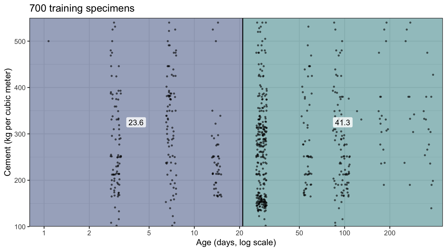
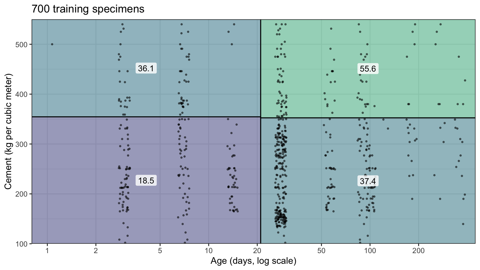
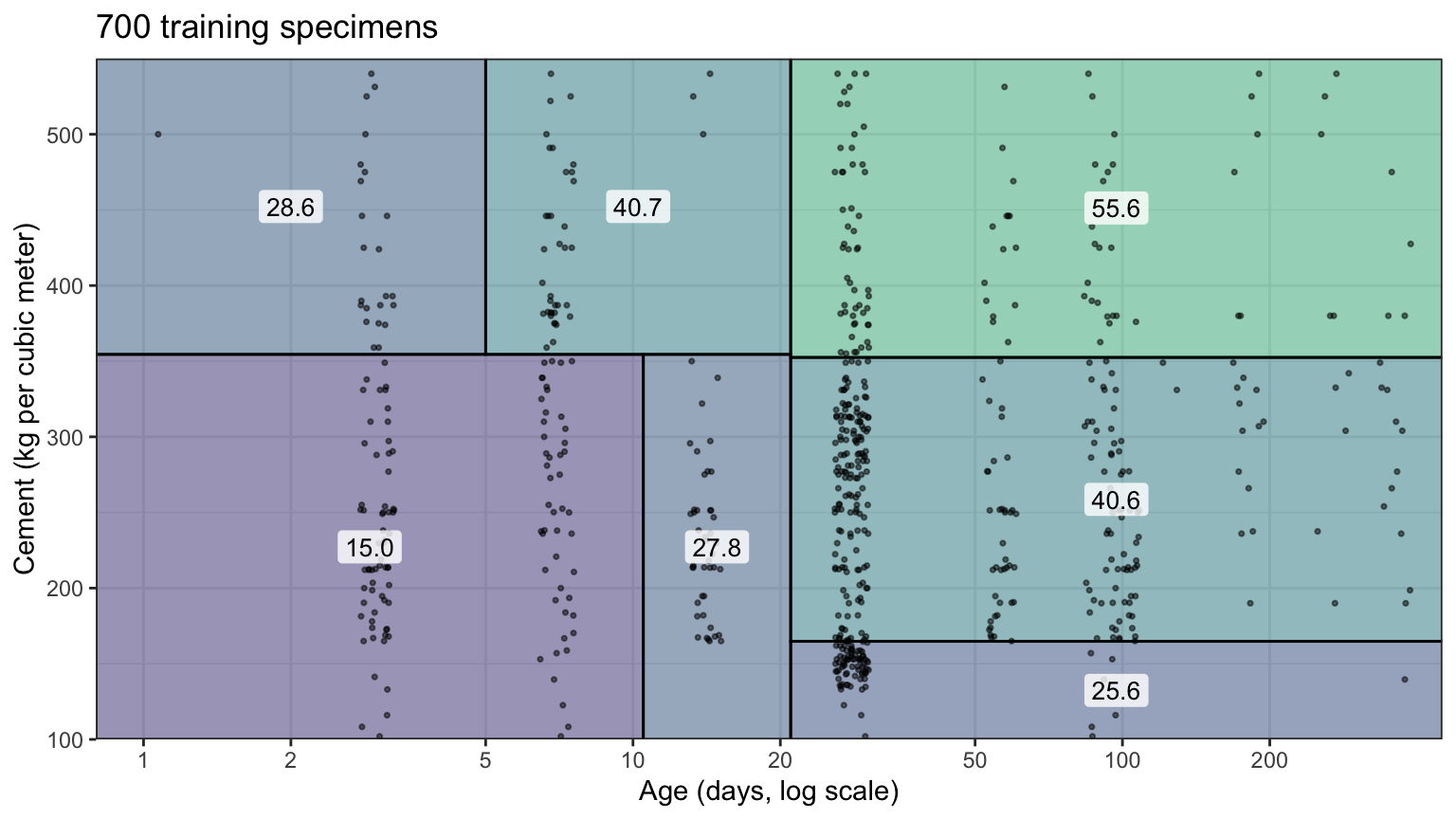
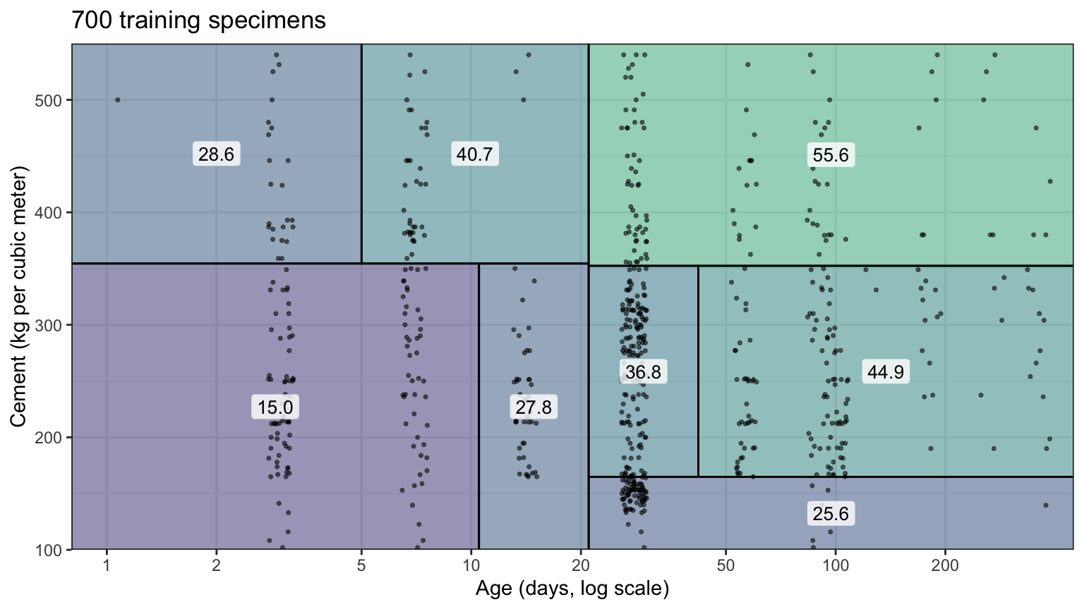
Pruning
Full tree
# The full tree: no threshold on the decrease in RSS, and leaves as small
# as one specimen.
full_control <- rpart.control(cp = 0, minsplit = 2, minbucket = 1)
full_fit <- rpart(compressive_strength ~ age + cement, data = train,
                  control = full_control)

# Number of leaves.
c(leaves = sum(full_fit$frame$var == "<leaf>"))
leaves
564 Overfitting
Cost-complexity pruning
\[C_\alpha(T) = \sum_{\ell=1}^{|T|}\sum_{i:\, x_i \in R_\ell}\left(y_i - \widehat y_{R_\ell}\right)^2 + \alpha|T|,\]
- \(T\) — subtree of the full tree \(T_0\), some internal nodes turned into leaves
- \(|T|\) — number of leaves of \(T\); \(R_\ell\) — its \(\ell\)th leaf
- \(\alpha\) — tuning parameter, the RSS a leaf must remove to be worth keeping
- \(\alpha = 0\): the minimizer is \(T_0\); larger \(\alpha\), fewer leaves, down to the root alone
rpart():cpis \(\alpha\) divided by the RSS of the root
Cross-validation
            CP nsplit rel error    xerror       xstd
17 0.005262351     21 0.2978793 0.4307607 0.02853326
18 0.004928922     22 0.2926170 0.4226674 0.02808284
19 0.003547482     23 0.2876881 0.4076152 0.02743197
20 0.003334777     25 0.2805931 0.4134854 0.02712277
21 0.003269014 26 0.2772583 0.4204379 0.02827351Cross-validation curve
Pruned tree
# Prune the full tree at the cp with the smallest xerror.
cp_best <- cp_table[best_row, "CP"]
pruned_fit <- prune(full_fit, cp = cp_best)

# Test MSE of the full and the pruned tree.
y_test <- test$compressive_strength
c(full = mean((y_test - predict(full_fit, test))^2),
  pruned = mean((y_test - predict(pruned_fit, test))^2))
full pruned
136.3742 111.5602 Pruned tree regions
All explanatory variables
| Method | Leaves, age and cement | Test MSE, age and cement | Leaves, all 8 | Test MSE, all 8 |
|---|---|---|---|---|
| Least squares | none | 172.7 | none | 106.4 |
| Default tree | 9 | 108.5 | 15 | 86.8 |
| Full tree | 564 | 136.4 | 659 | 40.3 |
| Pruned tree | 24 | 111.6 | 179 | 42.2 |
Classification trees
Penguin species
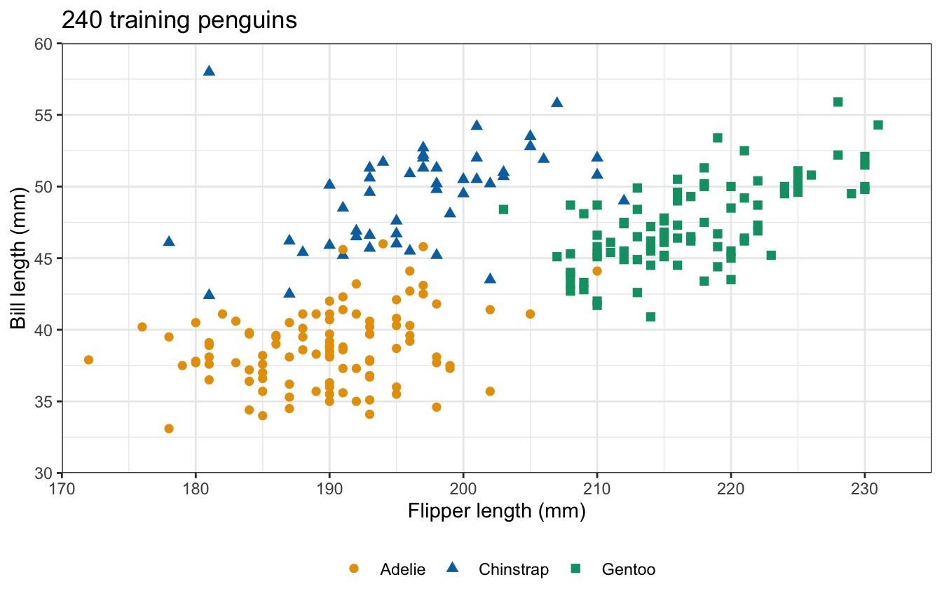
- Question: which of three species is a penguin, given four measurements of its body?
- Observation: a penguin
- Response variable:
species: Adelie, Chinstrap, Gentoo - Explanatory variables: bill length and bill depth (mm), flipper length (mm), body mass (g)
- Training sample: 240 penguins
- Test penguins: 102
Training penguins
Most common class
\[\widehat p_{\ell k} = \frac{1}{n_\ell}\sum_{i:\, x_i \in R_\ell}\mathrm{I}\left(y_i = k\right),\]
- \(K\) — number of classes, indexed \(k = 1, \ldots, K\)
- \(n_\ell\) — training observations in region \(R_\ell\)
- \(\widehat p_{\ell k}\) — proportion of them in class \(k\)
- Prediction for \(R_\ell\): the class \(k\) with the largest \(\widehat p_{\ell k}\)
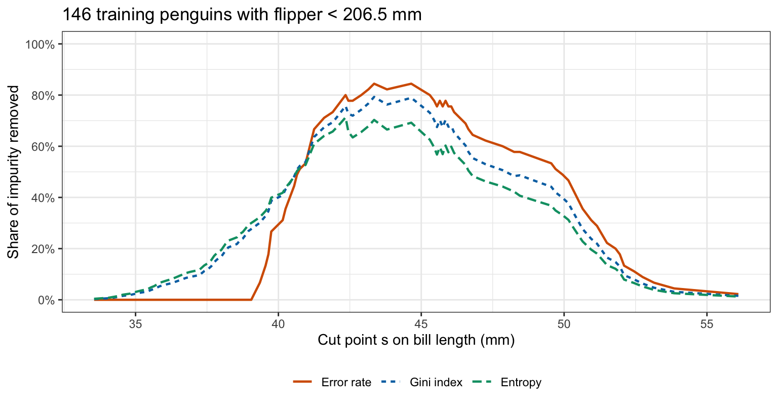
Node impurity
\[E_\ell = 1 - \max_k \widehat p_{\ell k}, \qquad G_\ell = \sum_{k=1}^K \widehat p_{\ell k}\left(1 - \widehat p_{\ell k}\right), \qquad D_\ell = -\sum_{k=1}^K \widehat p_{\ell k}\log \widehat p_{\ell k}\]
- \(E_\ell\) — classification error rate
- \(G_\ell\) — Gini index
- \(D_\ell\) — entropy, natural log, \(0\log 0 = 0\)
\[\frac{n_1 Q_1 + n_2 Q_2}{n_1 + n_2}\]
- Impurity of a split: \(Q\) is any of the three, \(Q_1\) and \(Q_2\) its values in the two regions
Impurity of a split
| Node | Adelie | Chinstrap | Gentoo | n | Error rate | Gini index | Entropy |
|---|---|---|---|---|---|---|---|
| Root | 102 | 48 | 90 | 240 | 0.575 | 0.639 | 1.053 |
| flipper < 206.5 | 101 | 44 | 1 | 146 | 0.308 | 0.431 | 0.651 |
| flipper >= 206.5 | 1 | 4 | 89 | 94 | 0.053 | 0.102 | 0.234 |
| Split (weighted) | 0.208 | 0.302 | 0.488 |
Gini index and entropy
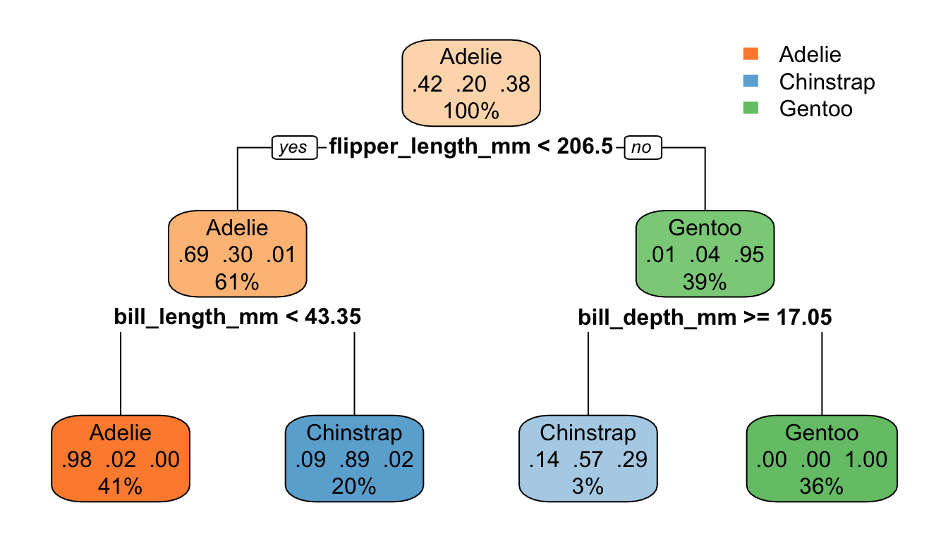
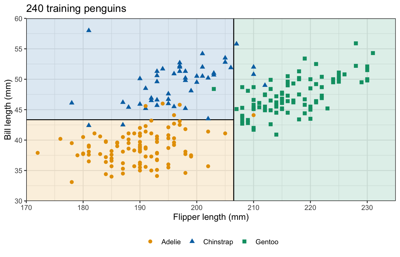
Fitting a classification tree
n= 240

node), split, n, loss, yval, (yprob)
      * denotes terminal node

1) root 240 138 Adelie (0.425000 0.200000 0.375000)
  2) flipper_length_mm< 206.5 146  45 Adelie (0.691781 0.301370 0.006849)
    4) bill_length_mm< 43.35 99   2 Adelie (0.979798 0.020202 0.000000) *
    5) bill_length_mm>=43.35 47   5 Chinstrap (0.085106 0.893617 0.021277) *
  3) flipper_length_mm>=206.5 94   5 Gentoo (0.010638 0.042553 0.946809)
    6) bill_depth_mm>=17.05 7   3 Chinstrap (0.142857 0.571429 0.285714) *
7) bill_depth_mm< 17.05 87 0 Gentoo (0.000000 0.000000 1.000000) *Fitted classification tree
Test confusion matrix
           Observed
Predicted   Adelie Chinstrap Gentoo
  Adelie        48         3      0
  Chinstrap      1        17      1
  Gentoo         0         0     32
[1] 0.9509804Pruning a classification tree
# The full classification tree, and its table from two rows above the
# smallest xerror.
penguin_full <- rpart(species ~ bill_length_mm + bill_depth_mm +
                        flipper_length_mm + body_mass_g,
                      data = penguin_train, method = "class",
                      control = full_control)
penguin_cp <- penguin_full$cptable
penguin_best <- which.min(penguin_cp[, "xerror"])
penguin_cp[max(1, penguin_best - 2):nrow(penguin_cp), ]
CP nsplit rel error xerror xstd
2 0.275362319 1 0.362318841 0.36231884 0.04559079
3 0.028985507 2 0.086956522 0.12318841 0.02879998
4 0.010869565 3 0.057971014 0.07246377 0.02243258
5 0.007246377 5 0.036231884 0.07246377 0.02243258
6 0.003623188 9 0.007246377 0.07971014 0.02347629
7 0.000000000 11 0.000000000 0.07246377 0.02243258Strengths and weaknesses
Interpretability
- Default concrete tree on age and cement: 9 leaves
- Default penguin tree: 4 leaves
- Any number of classes, no change to the method
- Pruned tree on all 8 explanatory variables: 179 leaves
Nonlinearity and interactions
- Test MSE on all 8 explanatory variables: pruned tree 42.2, least squares 106.4
- Least squares with \(\log(\texttt{age})\) in place of age: 48.5
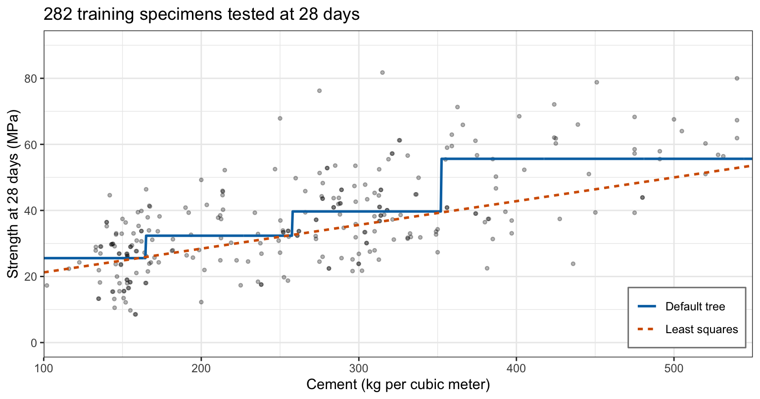
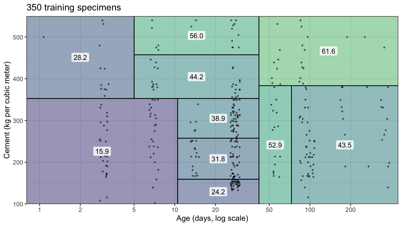
- Default tree on age and cement: younger than 21 days, cement split at 354.5; older, at 164.8, 257.7 and 352.5
Step functions
Instability
Conclusion
- A tree predicts a constant in each rectangle: the mean, or the most common class
- Recursive binary splitting is greedy and top-down
- Gini index or entropy, not the error rate, grows a classification tree
- Cross-validated pruning sets the size of the tree
- Small trees are readable and capture nonlinearity and interactions
- Predictions are step functions with high variance
DS 3030