Boosting

Today

  • Data
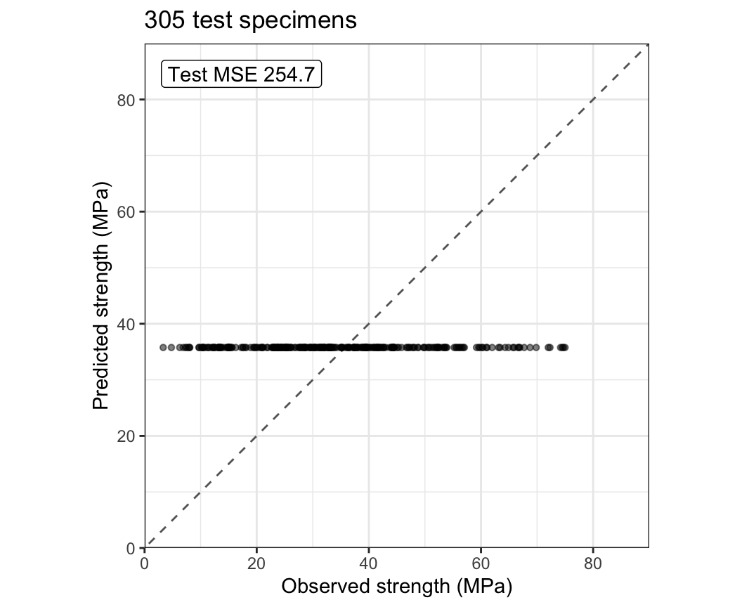
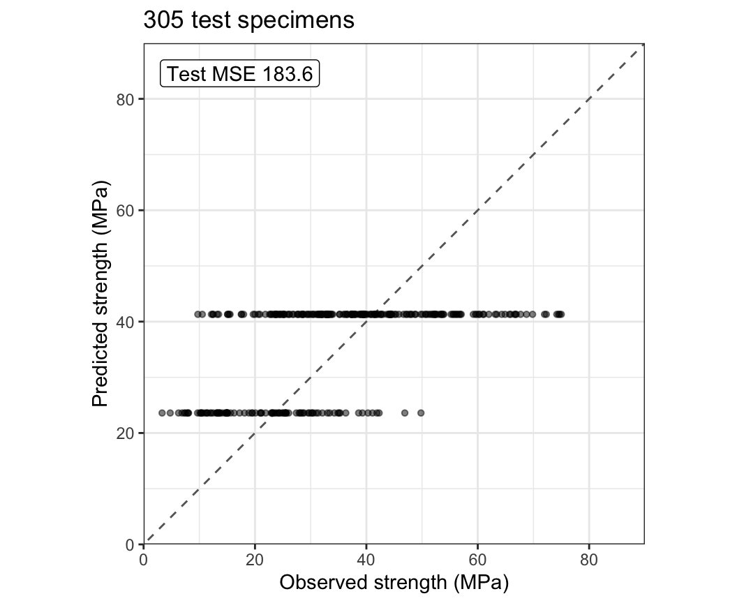
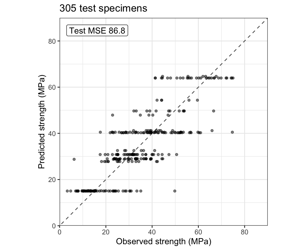
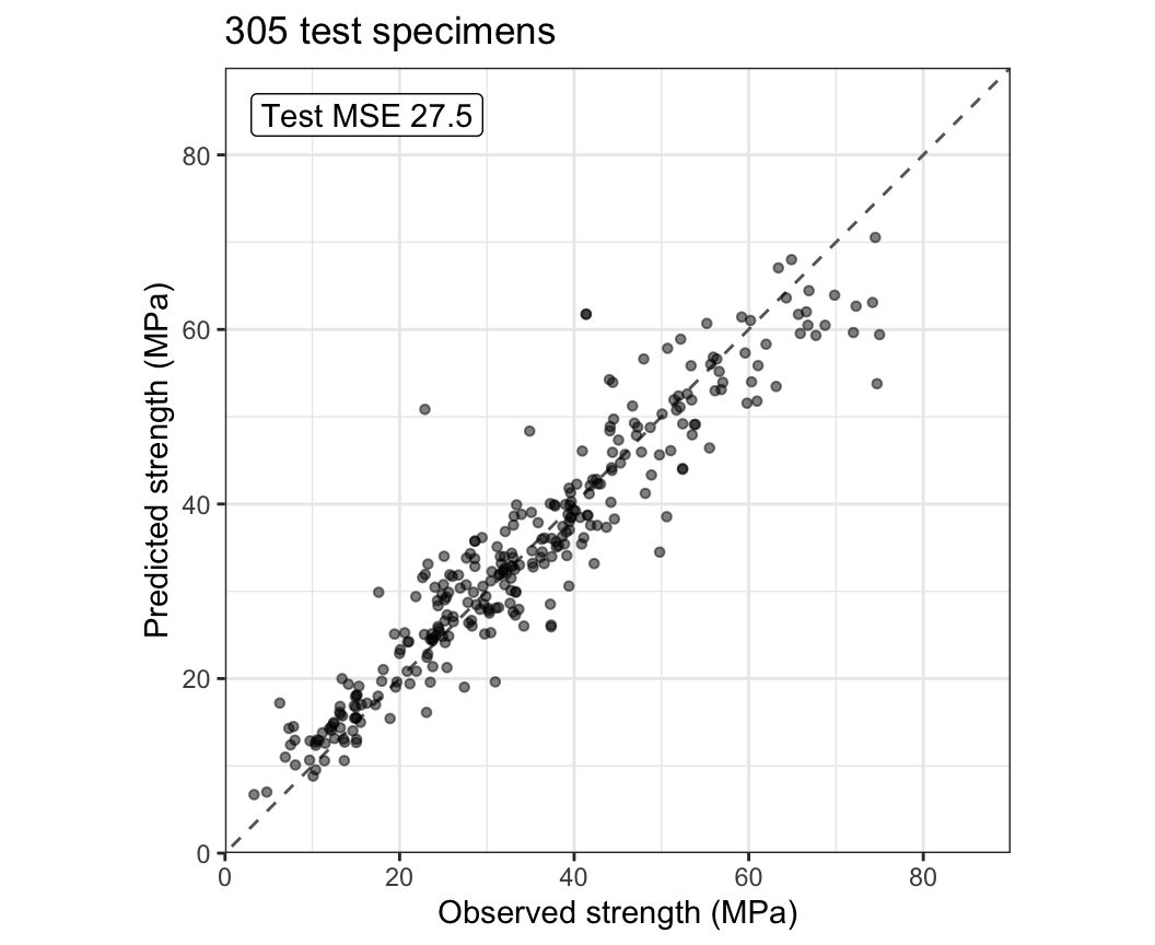
    • Earlier fits
  • Boosting
    • Main ideas
    • Algorithm
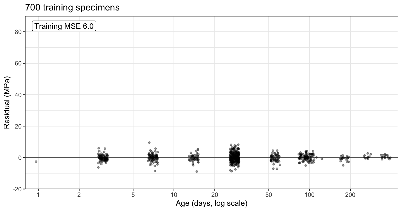
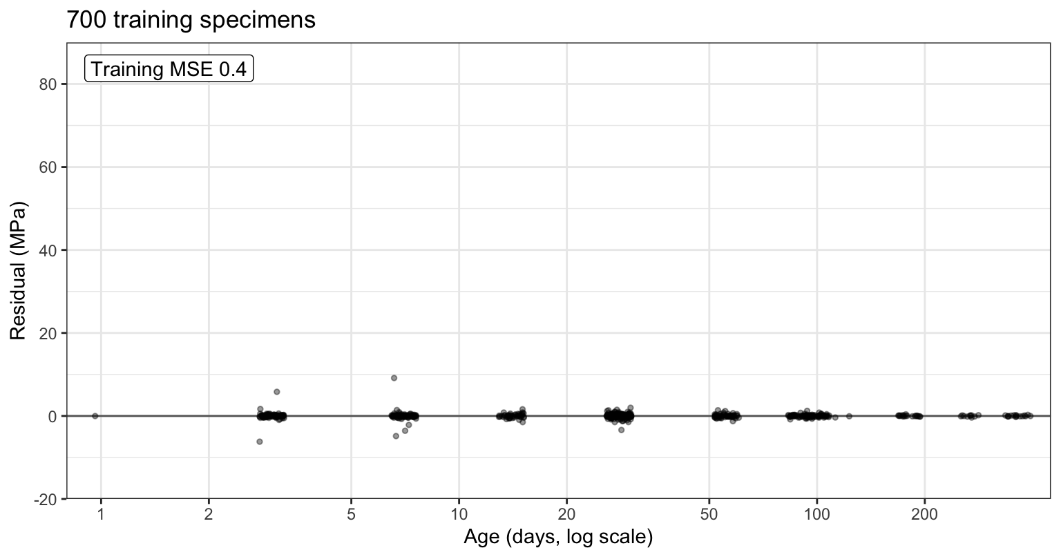
    • Residuals
    • Loop using rpart()
    • xgboost
    • Leaf predictions
    • Loop reproduction
  • Tuning parameters
    • Tuning parameters
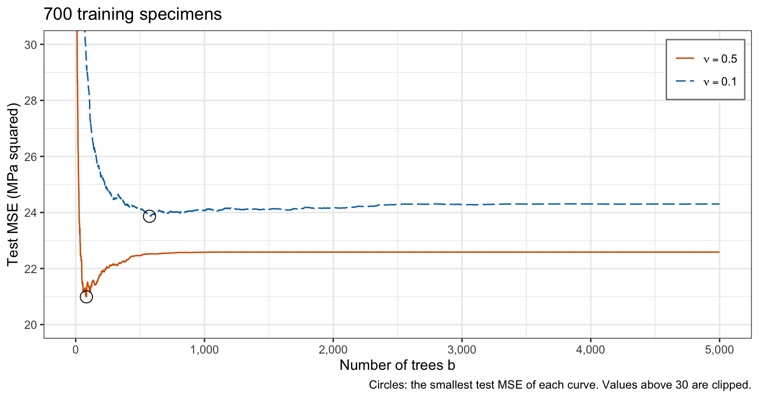
    • Shrinkage
    • Tree depth
    • Overfitting
    • Cross-validation estimate
    • Chosen model
    • Test error
  • Variable importance
    • RSS decrease
    • Forest and tree importance
    • Interpretation
  • Additive structure
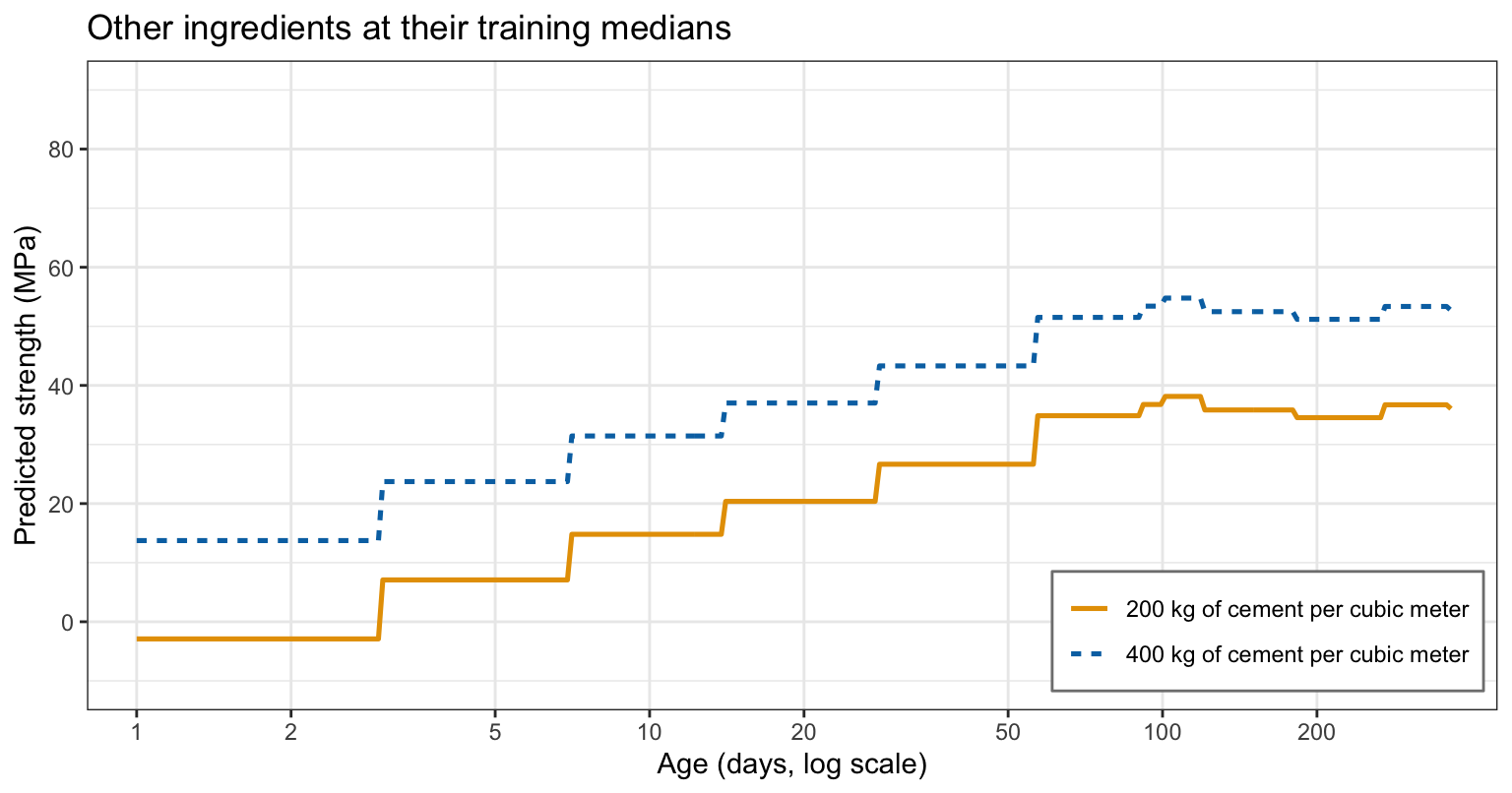
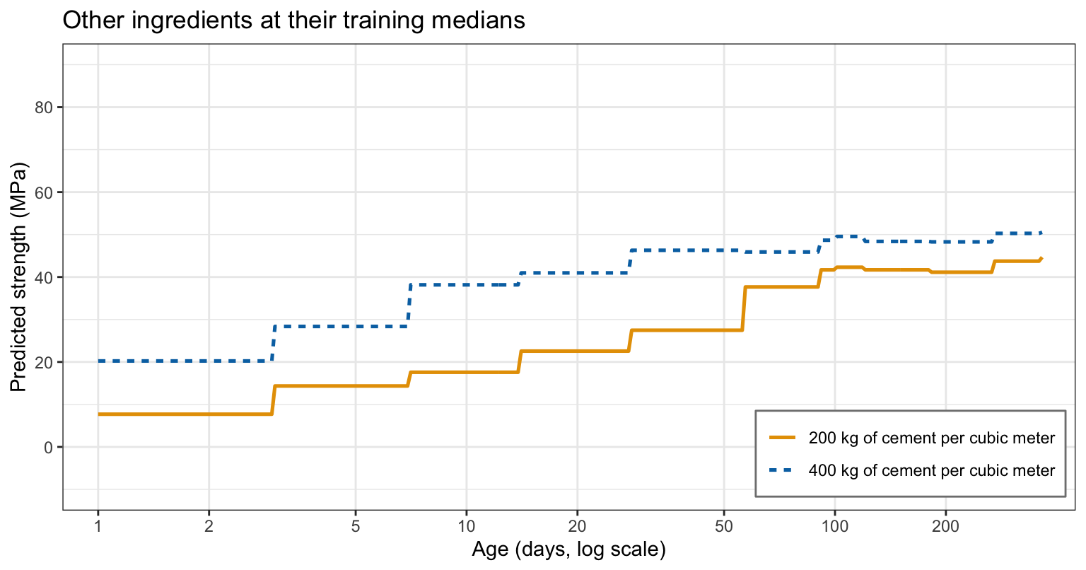
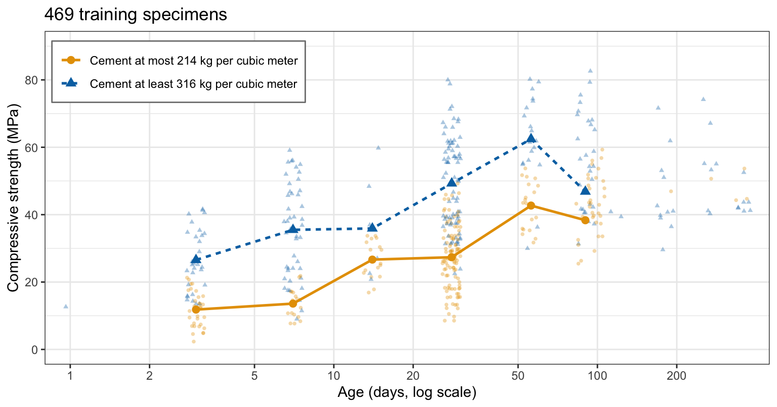
    • Cement and age
    • Stumps
    • Depth and interactions
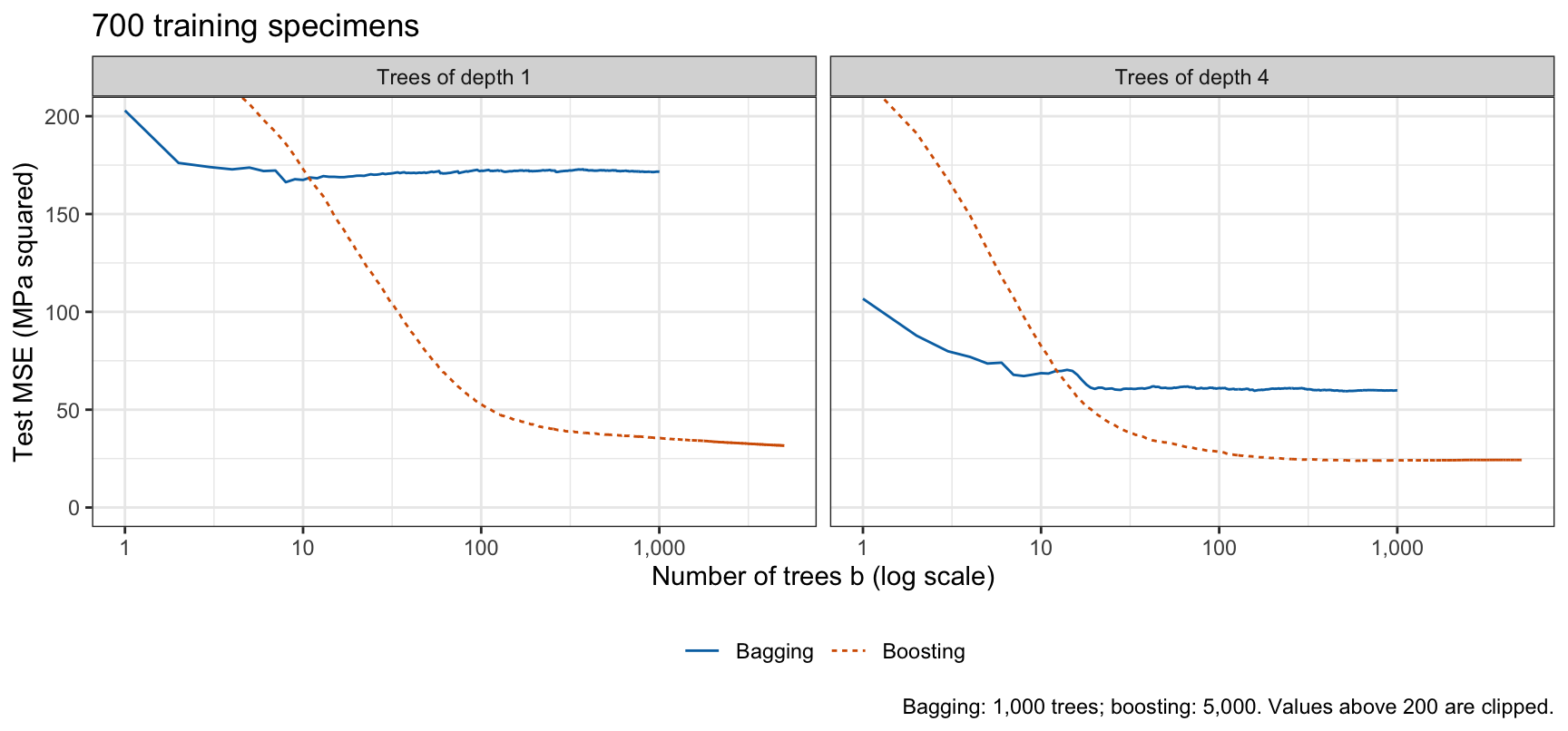
  • Comparison
    • Bias and variance
    • Limits

Data

Concrete specimens

  • Response: compressive_strength
  • Explanatory variables (\(p = 8\)):
    • cement
    • blast_furnace_slag
    • fly_ash
    • water
    • superplasticizer
    • coarse_aggregate
    • fine_aggregate
    • age
  • Training specimens: 700
  • Test specimens: 305

Earlier fits

Boosting

Main ideas

  • Sequentially build small trees
  • Fit each tree to the residuals
  • Prediction:
    • Sum of the trees’ predictions
    • Each times a small shrinkage \(\nu\)

Algorithm

  1. Set \(\widehat f_0(x) = 0\) and \(r_i = y_i\) for \(i = 1, \ldots, n\).
  2. For \(b = 1, \ldots, B\):
    1. fit a tree \(\widehat f^b\) of depth \(\delta\) to the residuals \(r_1, \ldots, r_n\);
    2. add a shrunken copy of it to the fit, \(\widehat f_b(x) = \widehat f_{b-1}(x) + \nu\,\widehat f^b(x)\);
    3. update the residuals, \(r_i \leftarrow r_i - \nu\,\widehat f^b(x_i)\), so that \(r_i = y_i - \widehat f_b(x_i)\).
  3. Predict with the boosted model \(\widehat f_B(x) = \sum_{b=1}^B \nu\,\widehat f^b(x)\).
  • \(x_i\), \(y_i\) — explanatory variables and response of observation \(i\); \(n\) — number of observations
  • \(B\) — number of trees, indexed \(b\)
  • \(\widehat f^b(x)\) — prediction at \(x\) of the \(b\)th tree; \(\widehat f_b(x)\) — boosted model after \(b\) trees
  • \(\nu\), \(0 < \nu \le 1\) — shrinkage (learning rate)
  • \(\delta\) — depth of each tree; \(\delta = 1\) is a stump
  • \(r_i\) — current residual of observation \(i\)

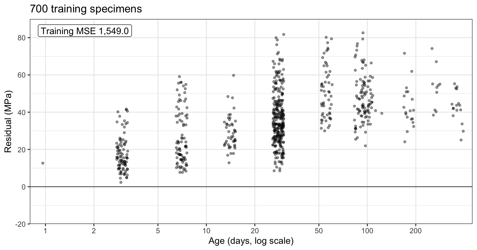
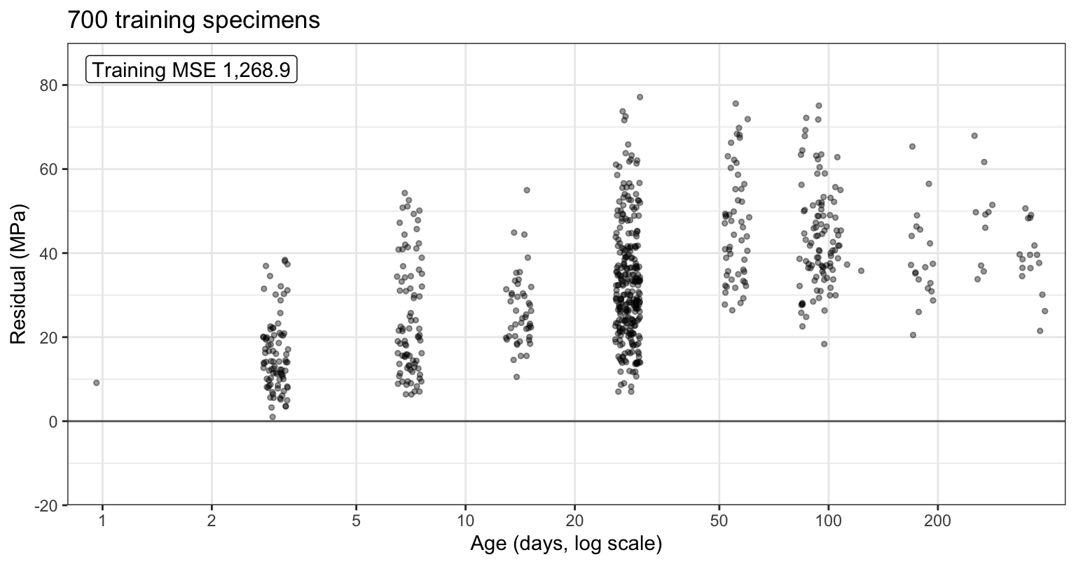
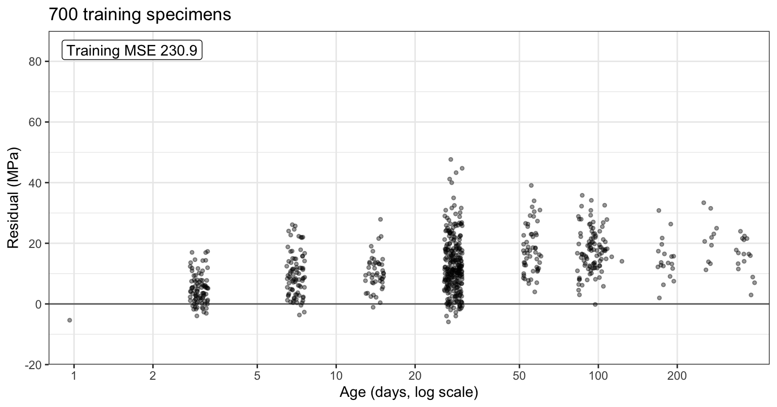
Residuals

Loop using rpart()

# Boosting from scratch: B trees of depth 4, with shrinkage nu.
B <- 1000
nu <- 0.1

# Start from the fit 0, so the residuals are the strengths.
r <- y_train
trees <- vector("list", B)

# Fit a tree to the residuals, then subtract nu times its predictions.
for (b in seq_len(B)) {
  data_b <- mutate(x_train, r = r)
  trees[[b]] <- rpart(r ~ ., data = data_b, control = small)
  r <- r - nu * predict(trees[[b]], x_train)
}

xgboost

# The training and test data in xgboost's format.
x_test <- select(test, -compressive_strength)
d_train <- xgb.DMatrix(x_train, label = y_train, nthread = 1)
d_test <- xgb.DMatrix(x_test, label = y_test, nthread = 1)

# B = 1,000 trees of depth 4 with shrinkage 0.1, and the test MSE.
params <- xgb.params(learning_rate = 0.1, max_depth = 4, nthread = 1)
fit <- xgb.train(params, d_train, nrounds = 1000)
mean((y_test - predict(fit, d_test))^2)
[1] 24.0684

Leaf predictions

\[\frac{\sum_{i \in \text{leaf}} r_i}{n_{\text{leaf}} + \texttt{lambda}},\]

  • the sum runs over the training specimens in the leaf
  • \(n_{\text{leaf}}\) — their number
  • lambda — penalty that shrinks the leaf’s prediction toward 0; default 1

Loop reproduction

Fit Settings Training MSE Test MSE
Loop of rpart() fits start at 0 0.42 23.7
xgboost, loop settings lambda = 0, base_score = 0, tree_method = "exact" 0.41 25.0
xgboost, defaults lambda = 1, start at the mean, tree_method = "hist" 0.58 24.1

Tuning parameters

Tuning parameters

  • Number of trees \(B\) (nrounds) — how many trees are added
  • Shrinkage \(\nu\) (learning_rate) — how fast the model learns
  • Depth \(\delta\) (max_depth) — how complex each tree is
  • Other xgboost settings (lambda, min_child_weight, gamma, subsample): defaults
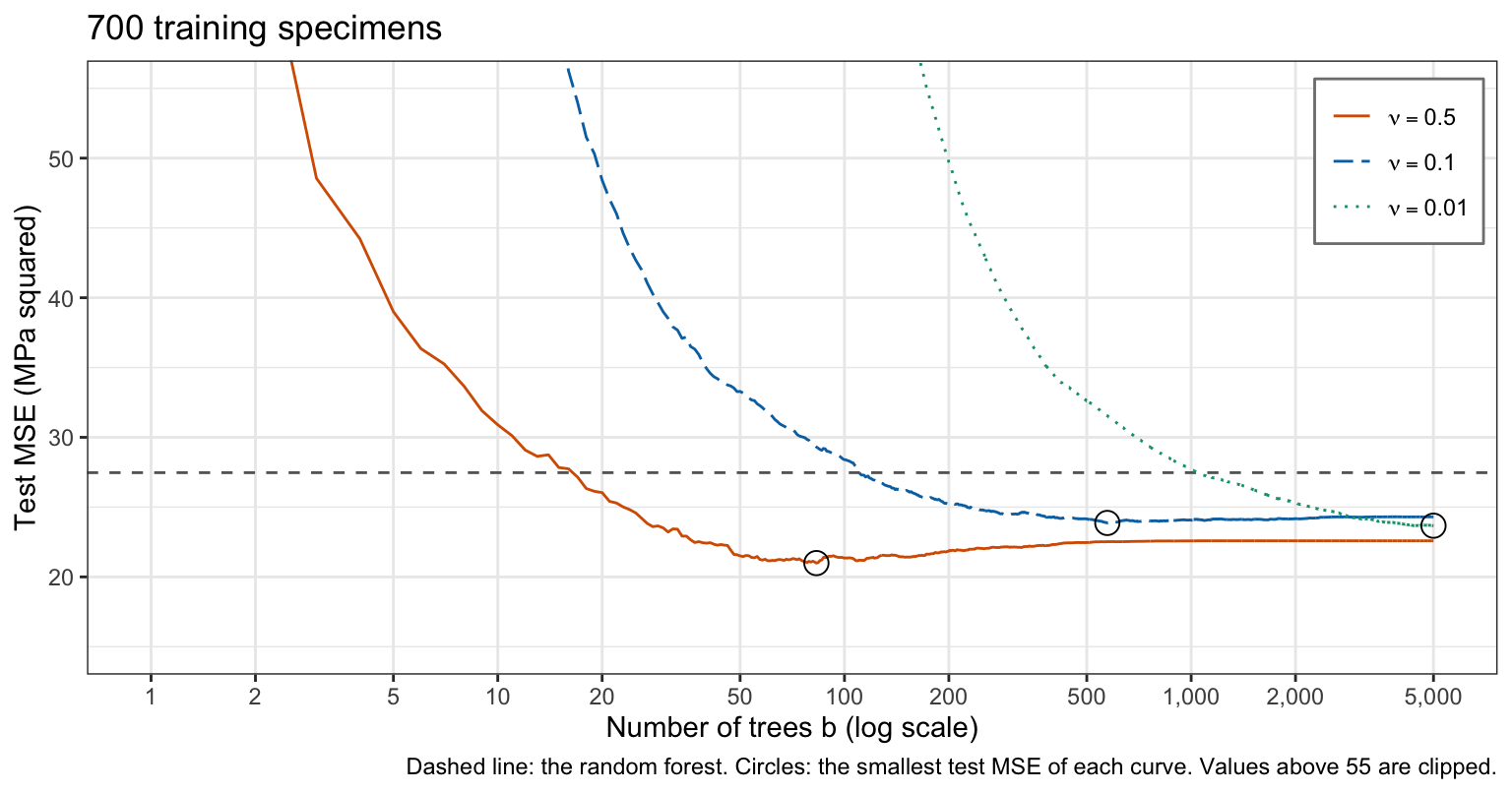
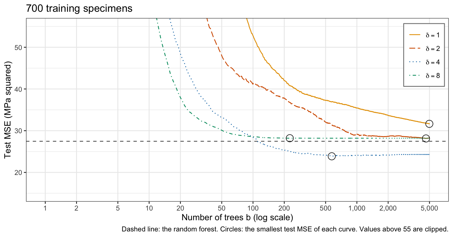
  • \(\nu = 0.1\) and \(\delta = 4\) fixed in advance; the next plots illustrate each parameter and choose nothing

Shrinkage

Tree depth

Overfitting

Cross-validation estimate

\[\text{CV}_{(10)}(B) = \frac{1}{10}\sum_{\ell=1}^{10}\text{MSE}_\ell(B), \qquad \text{MSE}_\ell(B) = \frac{1}{n_\ell}\sum_{i \in \mathcal{F}_\ell}\left[y_i - \widehat f_B^{(-\ell)}(x_i)\right]^2,\]

  • \(\mathcal{F}_\ell\) — training observations in fold \(\ell\); \(n_\ell\) — their number, \(n/10\)
  • \(\widehat f_B^{(-\ell)}\) — boosted model of \(B\) trees fit to the observations outside fold \(\ell\)
  • \(\text{MSE}_\ell(B)\) — its MSE on fold \(\ell\)

Cross-validation: RMSE

\[\text{CV}_{(10)}(B) = \frac{1}{10}\sum_{\ell=1}^{10}\text{RMSE}_\ell(B)^2 = \overline{\text{RMSE}}(B)^2 + \frac{9}{10}\,s_{\text{RMSE}}(B)^2,\]

  • \(\text{RMSE}_\ell(B)\) — root mean squared error on fold \(\ell\)
  • \(\overline{\text{RMSE}}(B)\) — mean over the folds of \(\text{RMSE}_\ell(B)\) (test_rmse_mean)
  • \(s_{\text{RMSE}}(B)\) — their standard deviation, divisor \(10 - 1 = 9\) (test_rmse_std)
  • Holds only when the folds have equal size (here 70 specimens each)
  • Used here because xgb.cv() records only the mean and standard deviation of the fold RMSEs

Cross-validation estimate in R

params: \(\nu = 0.1\) and \(\delta = 4\) fixed

# 10-fold cross-validation for every number of trees up to 5,000.
cv_fit <- xgb.cv(params, d_train, nrounds = 5000, nfold = 10, verbose = 0)
cv_log <- cv_fit$evaluation_log

# The CV estimate of the test MSE after each number of trees; the best B.
cv_mse <- cv_log$test_rmse_mean^2 + 0.9 * cv_log$test_rmse_std^2
B_cv <- which.min(cv_mse)
c(B = B_cv, cv = cv_mse[B_cv])
         B         cv 
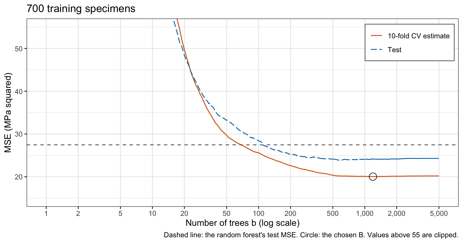
1194.00000   20.03447 
Chosen model

\(\nu = 0.1\), \(\delta = 4\), \(B = 1{,}194\)

Chosen model in R

\(\nu = 0.1\), \(\delta = 4\), \(B = 1{,}194\)

# The chosen model: B_cv trees, fit to all the training specimens.
fit_cv <- xgb.train(params, d_train, nrounds = B_cv)
mean((y_test - predict(fit_cv, d_test))^2)
[1] 24.14392

Test error

Method Tuning CV/OOB MSE Test MSE
Least squares, main effects none – 106.4
Least squares with log(age) none – 48.5
Default tree rpart() stopping rules – 86.8
Full tree none – 40.3
Pruned tree cp by 10-fold CV 60.8 42.2
Bagging, \(m = 8\) none 27.3 26.9
Random forest, \(m = 5\) \(m\) by OOB error 26.8 27.5
Boosting, \(\nu = 0.1\), \(\delta = 4\) \(\nu\) and \(\delta\) fixed in advance, \(B = 1{,}194\) by 10-fold CV 20.0 24.1

Variable importance

RSS decrease

\[\frac{n_1 n_2}{n_1 + n_2}\left(\bar r_1 - \bar r_2\right)^2,\]

  • \(n_1\), \(n_2\) — training specimens in the two parts of the node
  • \(\bar r_1\), \(\bar r_2\) — their mean residuals
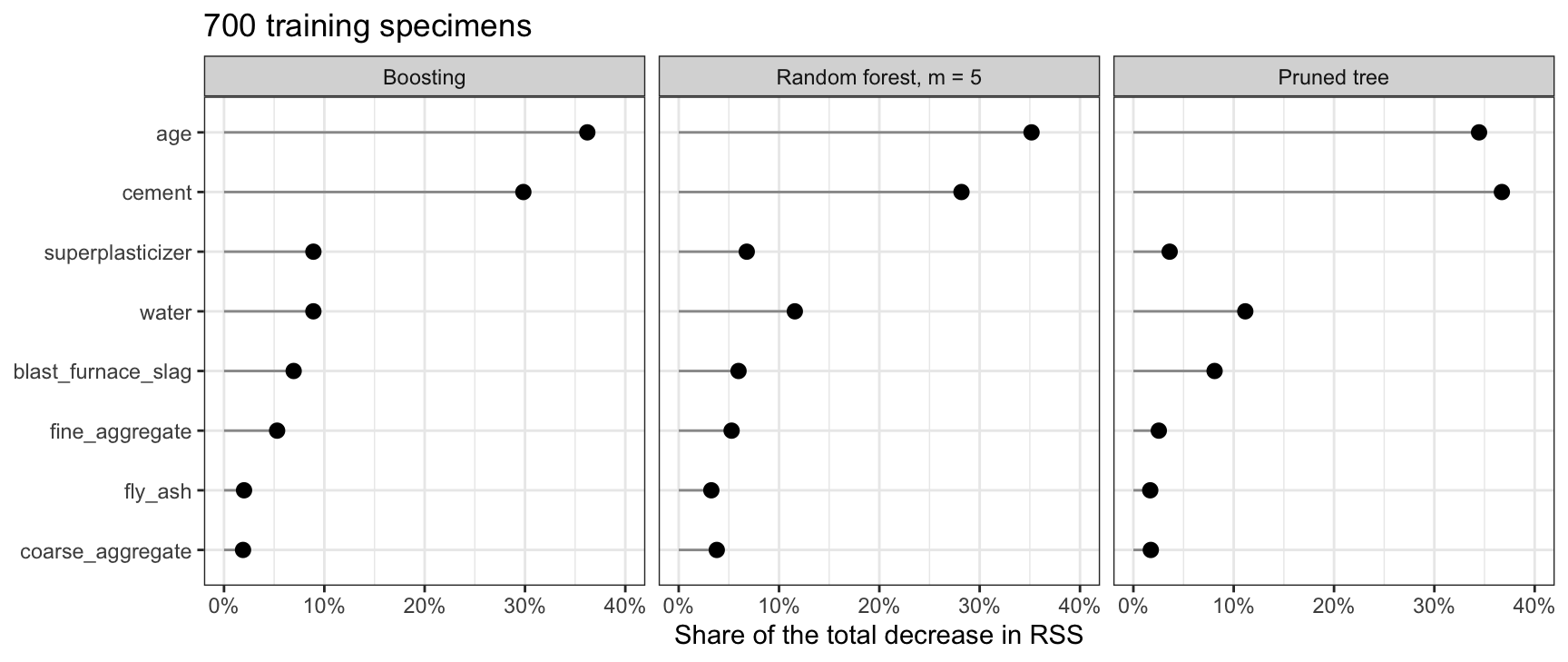
  • Importance of explanatory variable \(X_j\): the sum of these decreases over every split on \(X_j\) in all \(B\) trees, as a share of the total over the \(p\) variables
  • xgboost calls the decrease a split’s gain; the Gain column of xgb.importance() is each variable’s share

RSS decrease: gain

\[\text{gain} = \frac{S_1^2}{n_1 + \texttt{lambda}} + \frac{S_2^2}{n_2 + \texttt{lambda}} - \frac{S^2}{n_1 + n_2 + \texttt{lambda}},\]

  • \(S_1\), \(S_2\) — sums of the residuals in the two parts
  • \(S = S_1 + S_2\) — sum over the node
  • lambda — the leaf penalty of the Leaf predictions slide
  • lambda = 0: the gain equals the decrease in RSS

RSS decrease in R

# Each variable's share of the total gain of the chosen model's splits.
importance_boost <- xgb.importance(fit_cv)
importance_boost[, c("Feature", "Gain")]
              Feature       Gain
               <char>      <num>
1:                age 0.36214097
2:             cement 0.29837558
3:   superplasticizer 0.08909573
4:              water 0.08908287
5: blast_furnace_slag 0.06942685
6:     fine_aggregate 0.05293820
7:            fly_ash 0.01997255
8:   coarse_aggregate 0.01896725
Forest and tree importance

Interpretation

  • Importance ranks the variables
  • No direction
  • No effect size

Additive structure

Cement and age

Stumps

\[\widehat f_B(x) = \sum_{j=1}^p a_j(x), \qquad a_j(x) = \sum_{b:\, \widehat f^b \text{ splits on } X_j} \nu\,\widehat f^b(x),\]
  • \(a_j(x)\) — sum of the shrunken stumps that split on \(X_j\), a function of \(x\) only through \(X_j\)
  • Additive model: the change in the prediction when \(X_j\) changes does not depend on the other variables

Depth and interactions

  • Each leaf is reached through at most \(\delta\) splits
  • Interactions among at most \(\delta\) variables

Stumps and trees of depth 4

Comparison

Bias and variance

Limits

  • Three tuning parameters: \(B\), \(\nu\), \(\delta\); xgboost adds more, such as lambda
  • \(B\) must be chosen: too many trees overfit
  • Trees grown in sequence, not in parallel
  • No single tree to read
  • Predictions made of steps, constant beyond the largest training value

Conclusion

  • Boosting adds small trees, each fit to the residuals of the trees before it
  • xgboost starts from the mean and shrinks leaf predictions
  • A smaller \(\nu\) needs more trees; choose \(B\) by cross-validation
  • Importance ranks variables, with no direction or effect size
  • Depth \(\delta\) allows interactions among at most \(\delta\) variables
  • Boosting reduces bias; bagging reduces variance