Maximal Margin Classifier
Today
- Flea beetles
- Hyperplanes
- Equation
- Sides
- Signed distance
- Separating hyperplanes
- Class coding
- Separation condition
- Non-uniqueness
- Maximal margin
- Margin
- Optimization problem
- Best offset
- Best direction
- Fitting
- Estimates
- Support vectors
- Identification
- Refits
- Classification
- Sign rule
- Confidence
- Limitations
- Non-separable classes
- Sensitivity
Flea beetles
Flea beetles
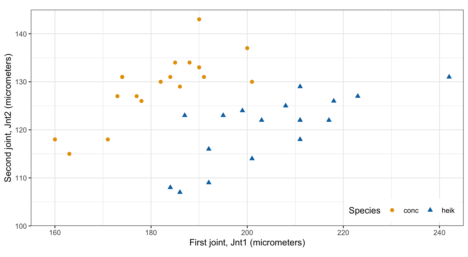
- Class:
Species(conc,heik) - Explanatory variables (\(p = 2\)):
Jnt1: first jointJnt2: second joint
- Beetles: 36 (18
conc, 18heik)
Flea beetles: plot
Hyperplanes
Equation
Hyperplane in \(p\) dimensions: the points \(X = (X_1, \ldots, X_p)^\top\) with
\[ \beta_0 + \beta_1 X_1 + \beta_2 X_2 + \cdots + \beta_p X_p = 0, \]
- \(X_j\) — value of feature \(j\), \(j = 1, \ldots, p\)
- \(\beta_0\) — intercept
- \(\beta = (\beta_1, \ldots, \beta_p)^\top\), not all zero — normal vector
- Dimension \(p - 1\): a line when \(p = 2\), a plane when \(p = 3\)
Sides
For any point \(x = (x_1, \ldots, x_p)^\top\), write
\[ f(x) = \beta_0 + \beta_1 x_1 + \cdots + \beta_p x_p = \beta_0 + \beta^\top x, \]
- \(f(x) = 0\): the hyperplane
- \(f(x) > 0\): the side \(\beta\) points toward
- \(f(x) < 0\): the other side
Sides: beetles
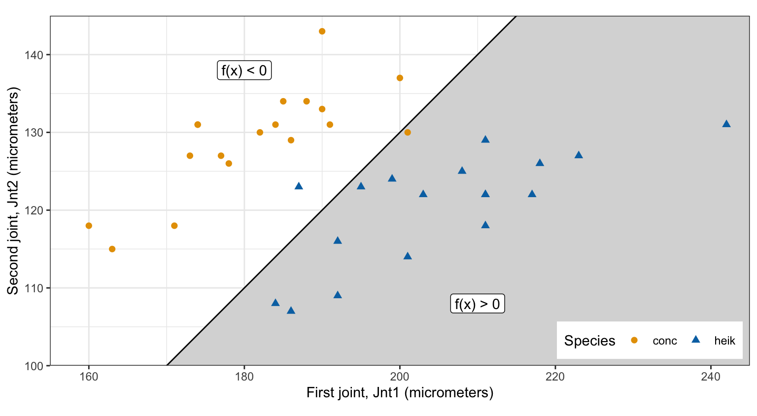
\(\beta_0 = -70\), \(\beta_1 = 1\), \(\beta_2 = -1\)
Signed distance
\[ t = \frac{f(x)}{\|\beta\|} = \frac{\beta_0 + \beta^\top x}{\|\beta\|}, \]
- \(t\) — signed distance from \(x\) to the hyperplane; its sign gives the side
- Unit normal vector, \(\|\beta\|^2 = \sum_{j=1}^p \beta_j^2 = 1\): \(t = f(x)\)
Separating hyperplanes
Class coding
\[ y_i = \begin{cases} 1 & \text{if observation } i \text{ is in one class,}\\ -1 & \text{if observation } i \text{ is in the other class,}\end{cases} \]
- \(i = 1, \ldots, n\) — training observation, with features \(x_i = (x_{i1}, \ldots, x_{ip})^\top\)
- Beetles: \(y_i = 1\) for
heik, \(y_i = -1\) forconc; \(n = 36\), \(p = 2\)
Separation condition
\[ y_i\left(\beta_0 + \beta_1 x_{i1} + \cdots + \beta_p x_{ip}\right) > 0 \quad \text{for all } i = 1, \ldots, n. \]
- \(y_i = 1\) needs \(f(x_i) > 0\); \(y_i = -1\) needs \(f(x_i) < 0\)
- Separable: some hyperplane satisfies this
Non-uniqueness
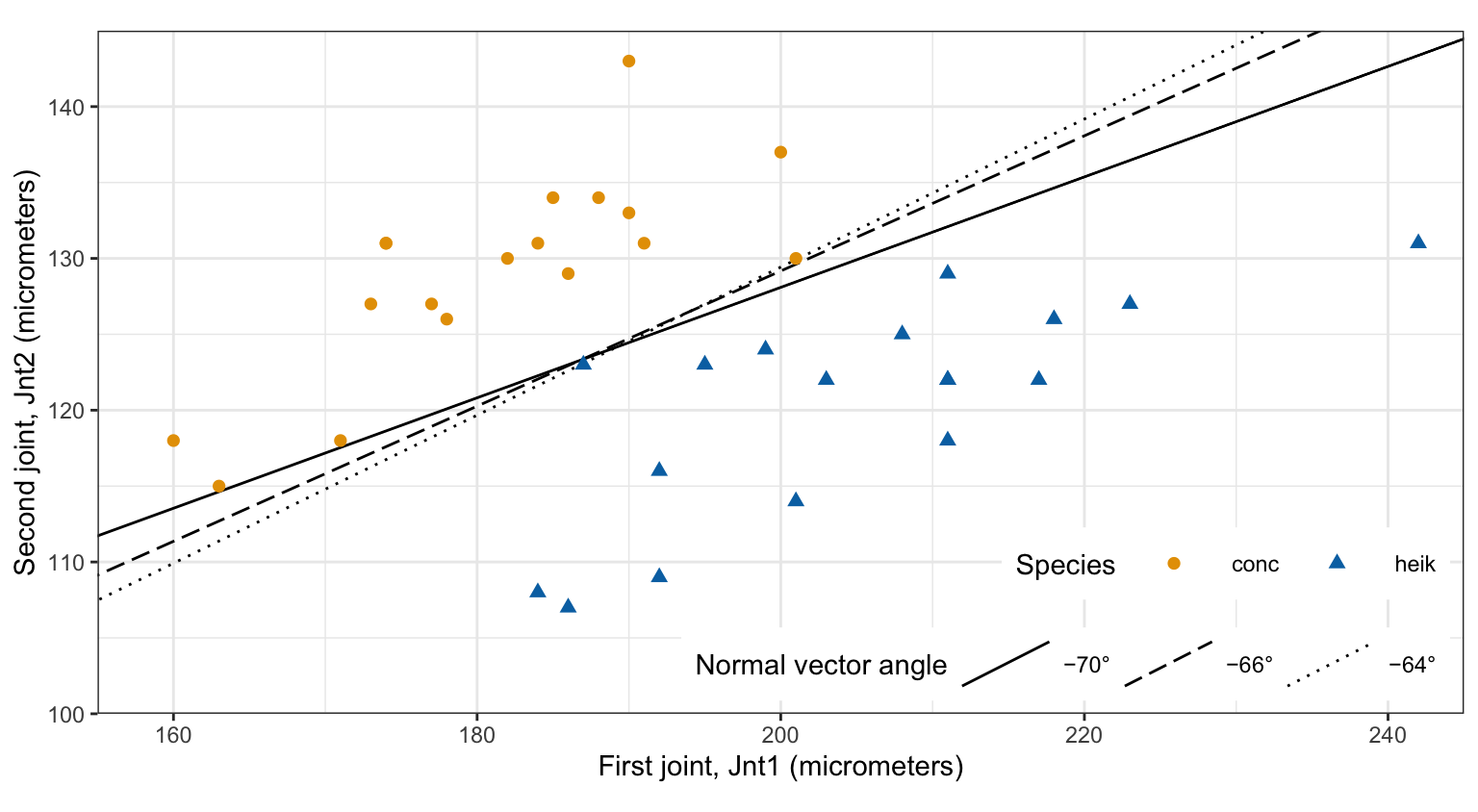
Legend: direction of \(\beta = (\cos\theta, \sin\theta)^\top\), by its angle \(\theta\) from the Jnt1 axis
Maximal margin
Margin
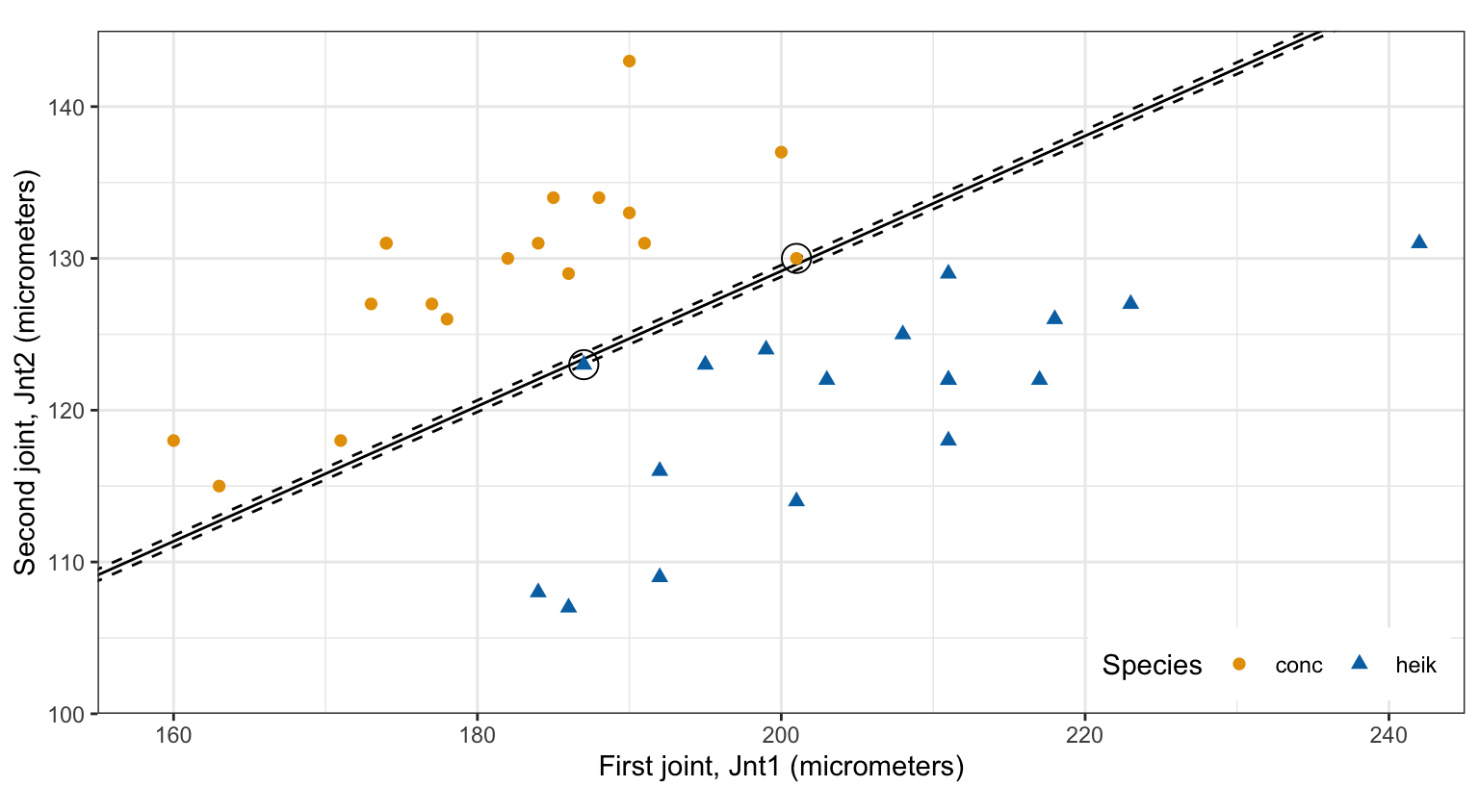
Margin \(= \min_i y_i f(x_i)\), with a unit normal vector
Optimization problem
Maximal margin hyperplane: the separating hyperplane with the largest margin
\[ \begin{aligned} \underset{\beta_0, \beta_1, \ldots, \beta_p, M}{\text{maximize}} \quad & M \\ \text{subject to} \quad & \sum_{j=1}^p \beta_j^2 = 1, \\ & y_i\left(\beta_0 + \beta_1 x_{i1} + \cdots + \beta_p x_{ip}\right) \ge M \quad \text{for all } i = 1, \ldots, n, \end{aligned} \]
- \(M\) — margin
- \(\sum_j \beta_j^2 = 1\): \(\beta_0 + \beta^\top x_i\) is the signed distance from \(x_i\) to the hyperplane
- \(y_i\left(\beta_0 + \beta^\top x_i\right) \ge M\): observation \(i\) on its own class’s side, at distance at least \(M\)
Best offset
Fixed unit normal vector \(\beta\):
\[ 2M \le \Delta(\beta) = \min_{i: y_i = 1}\beta^\top x_i - \max_{i: y_i = -1}\beta^\top x_i, \]
- \(\Delta(\beta)\) — gap between the classes along \(\beta\)
\[ \beta_0 = -\frac{1}{2}\left(\min_{i: y_i = 1}\beta^\top x_i + \max_{i: y_i = -1}\beta^\top x_i\right). \]
Best hyperplane: midway between the classes, margin \(\Delta(\beta)/2\)
Best direction
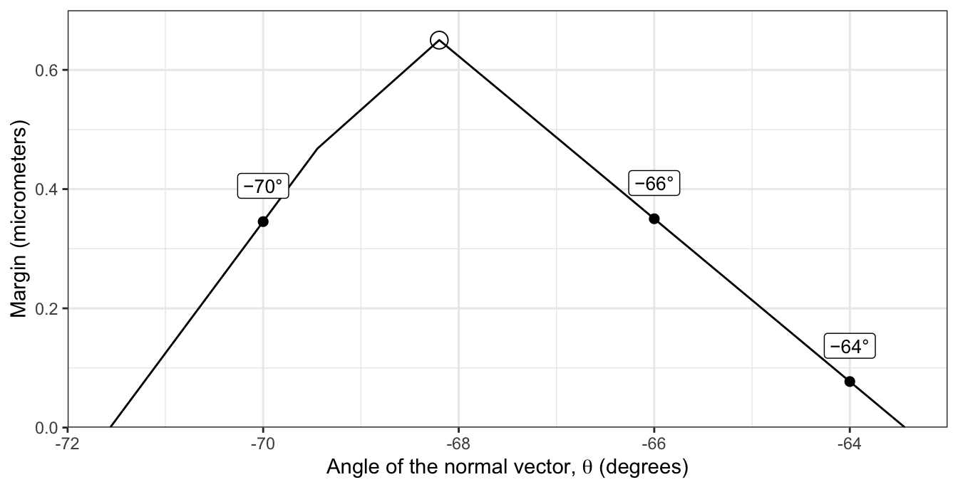
Fitting
Call:
svm(formula = Species ~ Jnt1 + Jnt2, data = beetles, kernel = "linear",
    cost = 1e+05, tolerance = 1e-08, scale = FALSE)


Parameters:
   SVM-Type:  C-classification
 SVM-Kernel:  linear
       cost:  1e+05

Number of Support Vectors: 3Estimates
\[ \widehat\beta_0 = \frac{\widehat w_0}{\|\widehat w\|}, \qquad \widehat\beta = \frac{\widehat w}{\|\widehat w\|}, \qquad \widehat M = \frac{1}{\|\widehat w\|}. \]
- \(w_0 = \beta_0/M\), \(w = \beta/M\): rescaled, so \(\|w\| = 1/M\) and \(y_i\left(w_0 + w^\top x_i\right) \ge 1\)
- \(\widehat w_0\) is
rho; \(-\widehat w\) is the weighted sum of the support vectors (rows ofSV, weightscoefs)
Estimates in R
# w and w0 with heik on the positive side (svm() makes the class of the
# first beetle, conc, positive).
w <- -drop(t(mmc_fit$coefs) %*% mmc_fit$SV)
w0 <- mmc_fit$rho

# Unit-norm estimates and the margin.
norm_w <- sqrt(sum(w^2))
beta_hat <- c(beta0 = w0, w) / norm_w
M_hat <- 1 / norm_w
round(c(beta_hat, M = M_hat), 4)
beta0 Jnt1 Jnt2 M
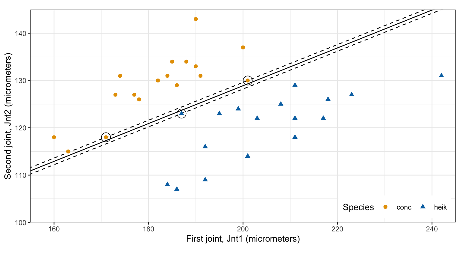
45.4025 0.3714 -0.9285 0.6499 Fitted hyperplane
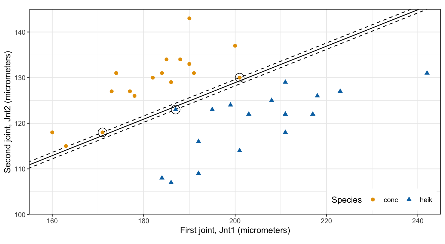
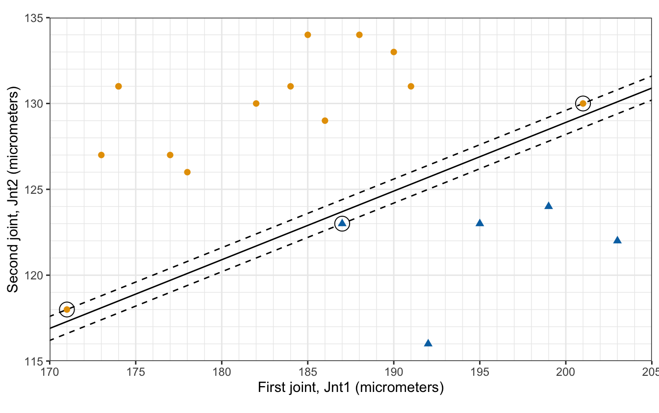
Support vectors
Identification
- Support vectors: observations on the margin, \(y_i \widehat f(x_i) = \widehat M\)
- The fitted hyperplane depends on the training data only through them
# Signed distance of each beetle, and its distance on its own side.
x_beetles <- as.matrix(beetles[c("Jnt1", "Jnt2")])
beetles <- beetles |>
  mutate(f_hat = drop(beta_hat["beta0"] + x_beetles %*% beta_hat[-1]),
         distance = y * f_hat)

# Beetles on the margin: distance M_hat, up to the solver's accuracy.
beetles |>
  filter(distance - M_hat < 1e-6) |>
  select(Specimen, Species, Jnt1, Jnt2, f_hat)
Specimen Species Jnt1 Jnt2 f_hat
1 5 conc 171 118 -0.6499337
2 13 conc 201 130 -0.6499337
3 35 heik 187 123 0.6499337Refits
| Beetles | \(n\) | \(\widehat\beta_0\) | \(\widehat\beta_1\) | \(\widehat\beta_2\) | \(\widehat M\) | Support vectors |
|---|---|---|---|---|---|---|
| All beetles | 36 | 45.4025 | 0.3714 | -0.9285 | 0.6499 | 5, 13, 35 |
| Without beetle 11 | 35 | 45.4025 | 0.3714 | -0.9285 | 0.6499 | 5, 13, 35 |
| Support vectors only | 3 | 45.4025 | 0.3714 | -0.9285 | 0.6499 | 5, 13, 35 |
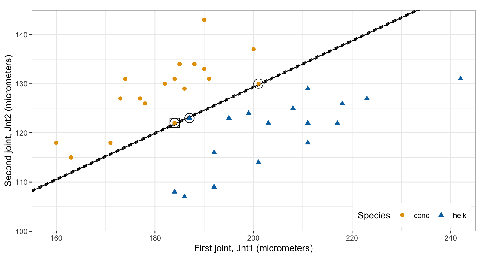
| Without beetle 13 | 35 | 3.4795 | 0.5450 | -0.8384 | 2.2638 | 1, 5, 35 |
Classification
Classification: new beetles
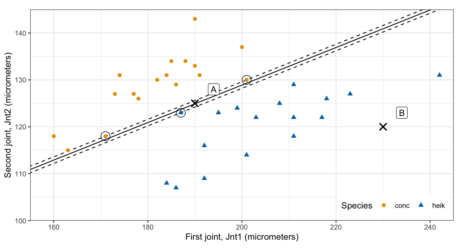
Sign rule
New beetle \(x^* = (x^*_1, \ldots, x^*_p)^\top\), classified by the sign of
\[ \widehat f(x^*) = \widehat\beta_0 + \widehat\beta_1 x^*_1 + \cdots + \widehat\beta_p x^*_p, \]
- \(\widehat f(x^*) > 0\): the class coded \(y = 1\)
- \(\widehat f(x^*) < 0\): the class coded \(y = -1\)
- A: \(\widehat f(x^*) = 45.4025 + 0.3714 \times 190 - 0.9285 \times 125 = -0.09\), so
conc - B: \(\widehat f(x^*) = 19.41\), so
heik
Confidence
- \(\left|\widehat f(x^*)\right|\) — distance from the new beetle \(x^*\) to the hyperplane, in micrometers
- Larger distance, more confident classification
- B: 19.41 micrometers; A: 0.09, less than \(\widehat M = 0.65\)
- A distance ranks confidence; it is not a probability
Limitations
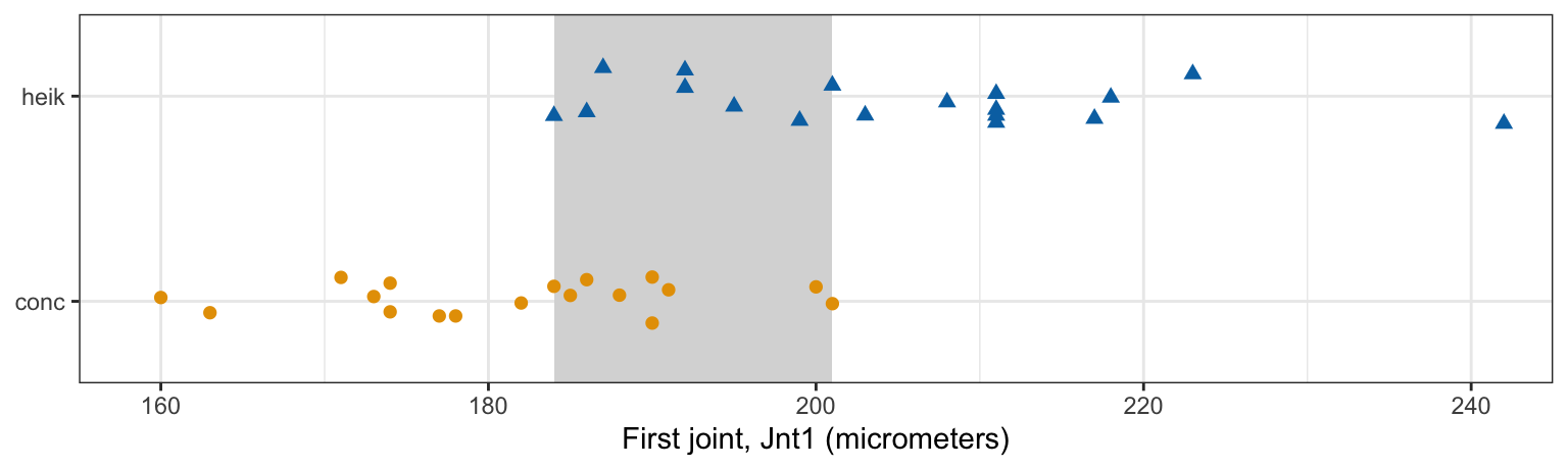
Non-separable classes
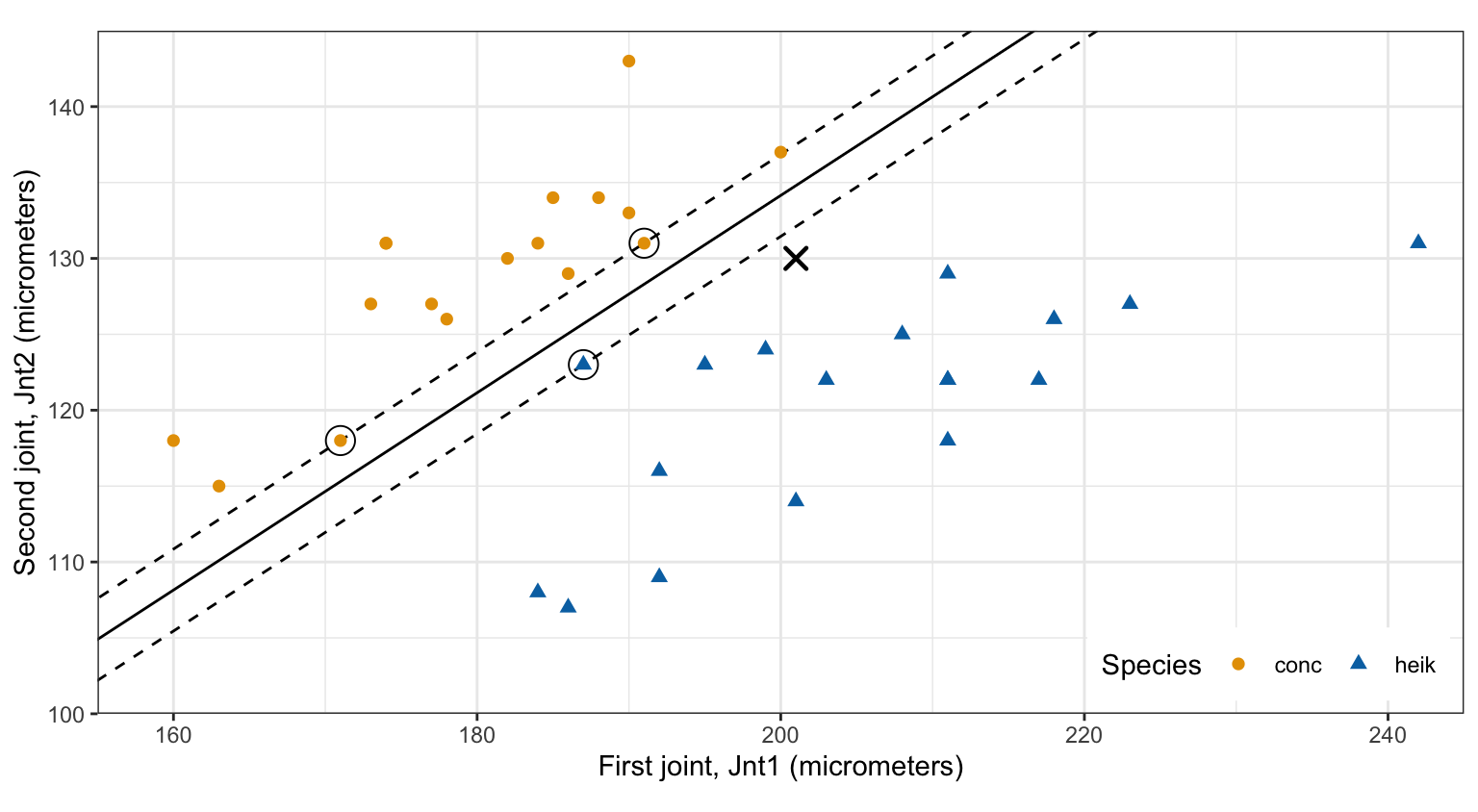
Sensitivity
Conclusion
- \(f(x)\): the side by its sign, the signed distance if \(\|\beta\| = 1\)
- Separable classes have infinitely many separating hyperplanes
- The maximal margin hyperplane has the largest margin
- The fit depends only on the support vectors
- No solution for overlapping classes; sensitive to single observations
- Next lecture: the support vector classifier
DS 3030