Support Vector Machines
Today
- Sacramento homes
- Enlarged feature space
- Polynomial features
- Feature count
- Kernels
- Inner products
- Kernel functions
- Polynomial kernel
- Radial kernel
- Fitting
- Tuning
- Grid
- Test error
- More than two classes
- One versus one and one versus all
- Pairwise voting
- Hinge and logistic loss
- Loss plus penalty
- Logistic loss
- Comparison
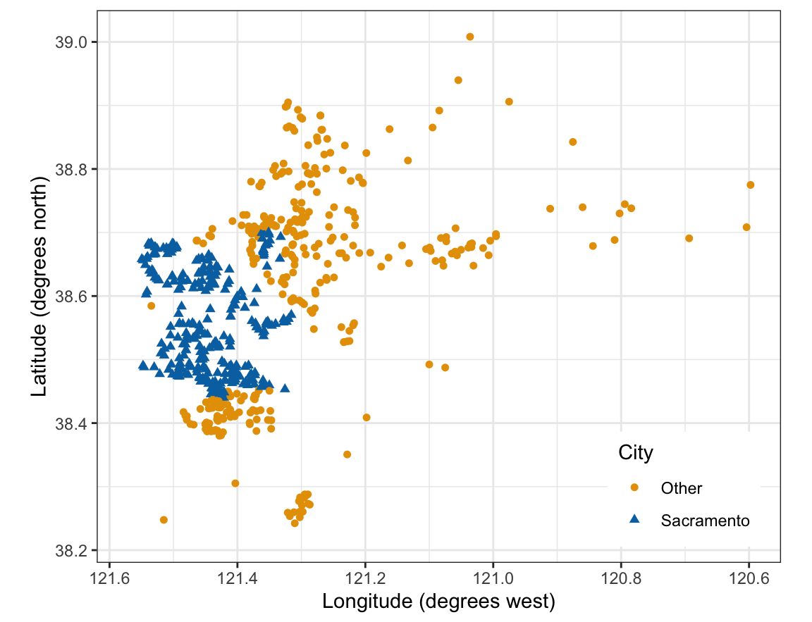
Sacramento homes
Sacramento homes
- Class:
place, the city (Sacramento: \(y = 1\),Other: \(y = -1\)) - Explanatory variables (\(p = 2\)):
longitude(degrees)latitude(degrees)
- Training homes: 621 (327
Other, 294Sacramento) - Test homes: 311
Sacramento homes: plot
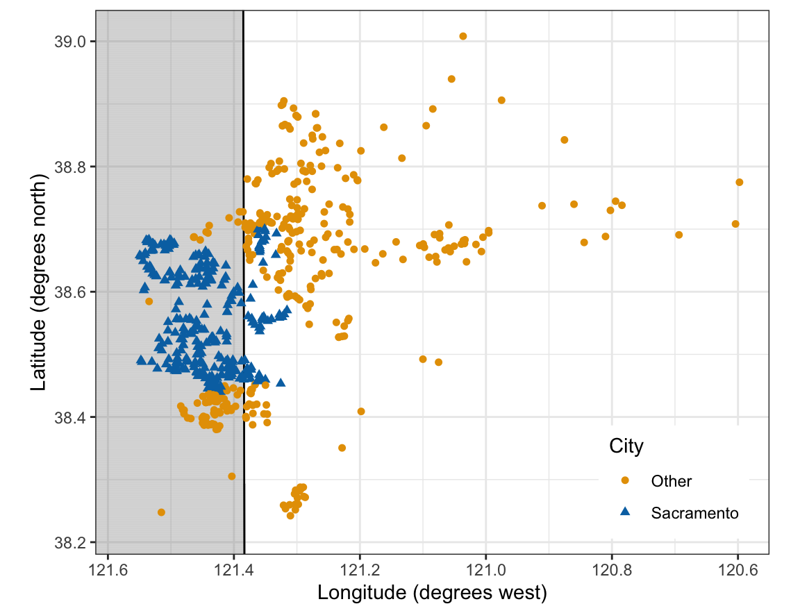
Enlarged feature space
Enlarged feature space
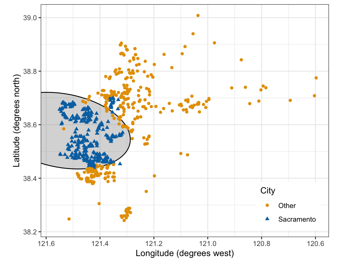
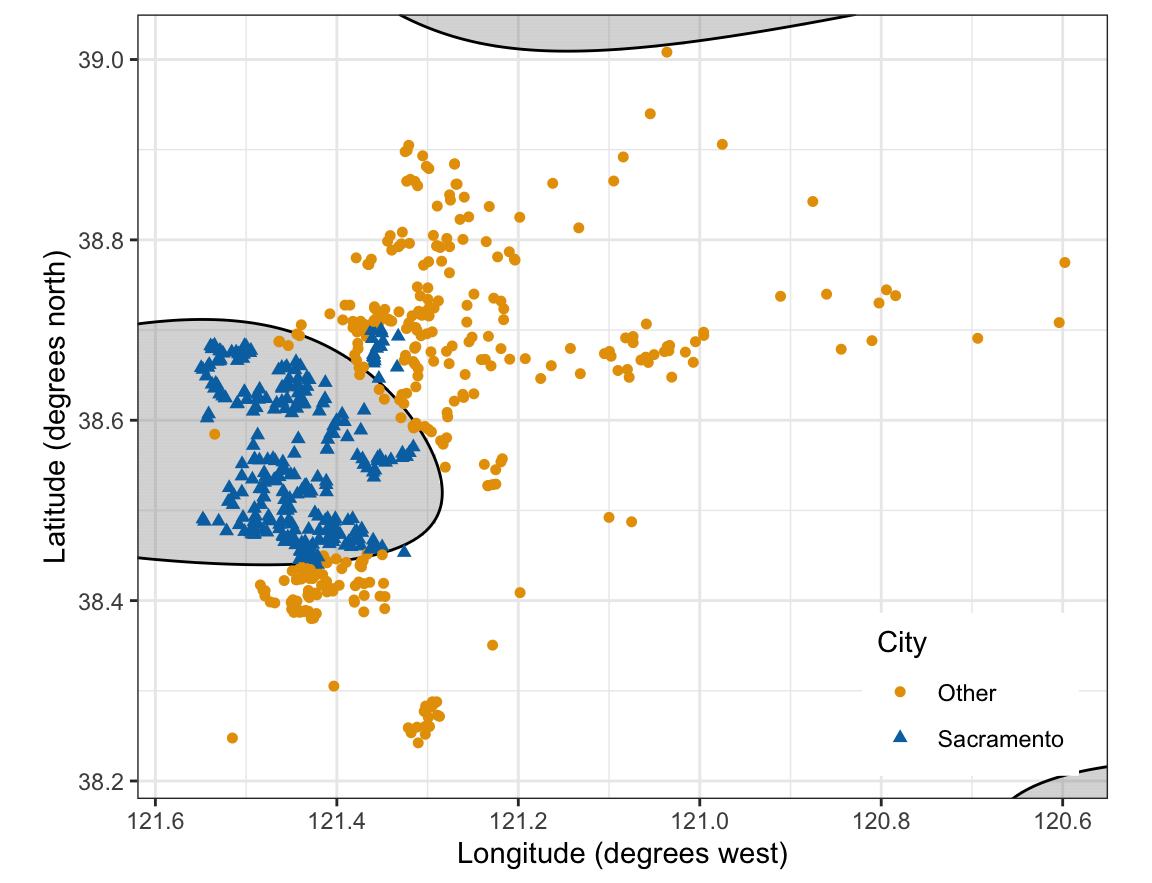
Polynomial features
Support vector classifier on the degree-2 features:
\[ \widehat w_0 + \widehat w_1X_1 + \widehat w_2X_2 + \widehat w_3X_1^2 + \widehat w_4X_1X_2 + \widehat w_5X_2^2 = 0 \]
- \(X_1, X_2\) — standardized longitude and latitude
- \(\widehat w_j\) — rescaled estimates, one per feature
- A hyperplane in five dimensions, a conic section in \(X_1\) and \(X_2\)
Polynomial features: fit
[1] 0.06602254Feature count
Monomials of degree at most \(d\) in \(p\) explanatory variables, without the constant:
\[ q = \binom{p + d}{d} - 1 \]
- \(q\) — number of features
- \(p = 2\): \(q = 5\) for \(d = 2\), \(q = 9\) for \(d = 3\)
- \(p = 10\): \(q = 285\) for \(d = 3\), \(q = 3{,}002\) for \(d = 5\)
Kernels
Inner products
\[ \widehat f(x) = \widehat w_0 + \sum_{i \in \mathcal{S}} \widehat\alpha_i \langle x, x_i\rangle, \]
- \(\mathcal{S}\) — set of support vectors
- \(\widehat\alpha_i\) — weight of support vector \(i\), positive for \(y_i = 1\), negative for \(y_i = -1\)
- \(\widehat w_0\) — rescaled intercept
- \(\langle x_i, x_{i'}\rangle = \sum_{j=1}^p x_{ij}x_{i'j}\) — inner product of two observations
Kernel functions
Support vector machine: the support vector classifier with a kernel
\[ f(x) = w_0 + \sum_{i \in \mathcal{S}} \alpha_i K(x, x_i). \]
- \(K(x_i, x_{i'})\) — kernel: a function of two observations that replaces the inner product
Kernel functions: three kernels
Linear (the inner product):
\[ K(x_i, x_{i'}) = \sum_{j=1}^p x_{ij}x_{i'j} \]
Polynomial of degree \(d\), a positive integer:
\[ K(x_i, x_{i'}) = \left(1 + \sum_{j=1}^p x_{ij}x_{i'j}\right)^d. \]
Radial, with \(\gamma > 0\):
\[ K(x_i, x_{i'}) = \exp\left(-\gamma\sum_{j=1}^p (x_{ij} - x_{i'j})^2\right). \]
Polynomial kernel
\(p = 2\) and \(d = 2\), expanding the square:
\[ \begin{aligned} \left(1 + x_{i1}x_{i'1} + x_{i2}x_{i'2}\right)^2 &= 1 + 2x_{i1}x_{i'1} + 2x_{i2}x_{i'2} + x_{i1}^2x_{i'1}^2 + 2x_{i1}x_{i2}x_{i'1}x_{i'2} + x_{i2}^2x_{i'2}^2 \\ &= \langle h(x_i), h(x_{i'})\rangle, \end{aligned} \]
where
\[ h(x_i) = \left(1,\ \sqrt2 x_{i1},\ \sqrt2 x_{i2},\ x_{i1}^2,\ \sqrt2 x_{i1}x_{i2},\ x_{i2}^2\right)^\top \]
- \(h(x_i)\) — degree-2 features of observation \(i\), up to constant multiples
Radial kernel
\[ \widehat f\left(x^*\right) = \widehat w_0 + \sum_{i \in \mathcal{S}}\widehat\alpha_i K\left(x^*, x_i\right) \]
- \(x^*\) — new observation; \(x_i\) — support vector \(i\)
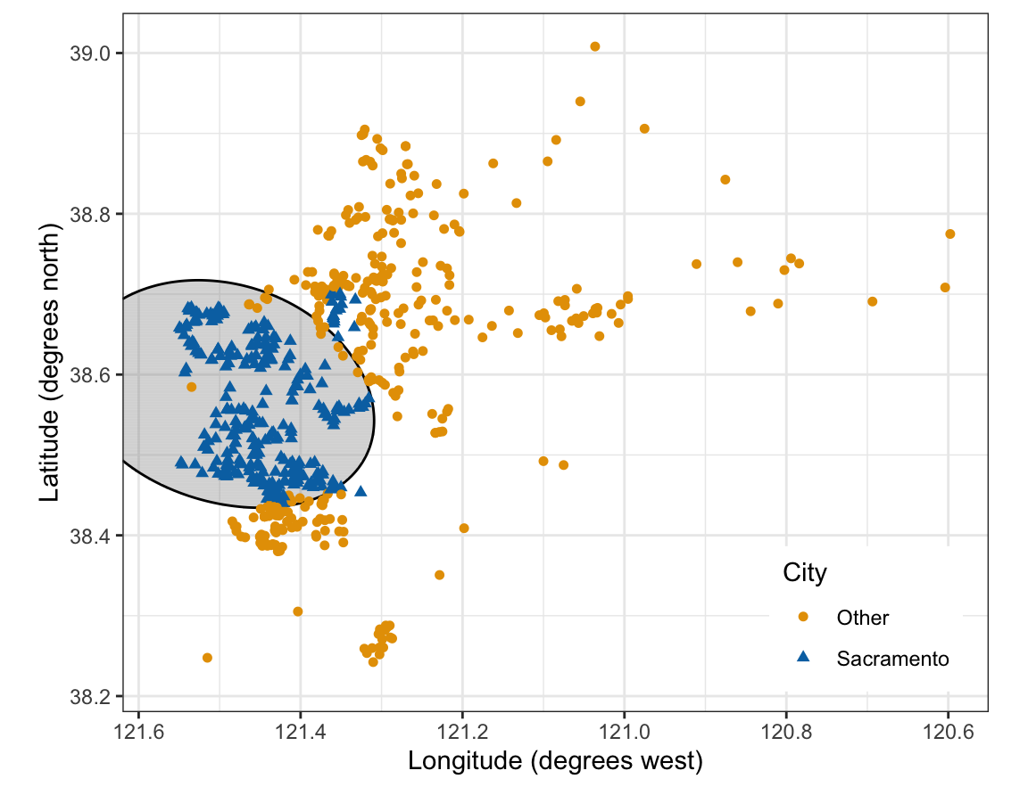
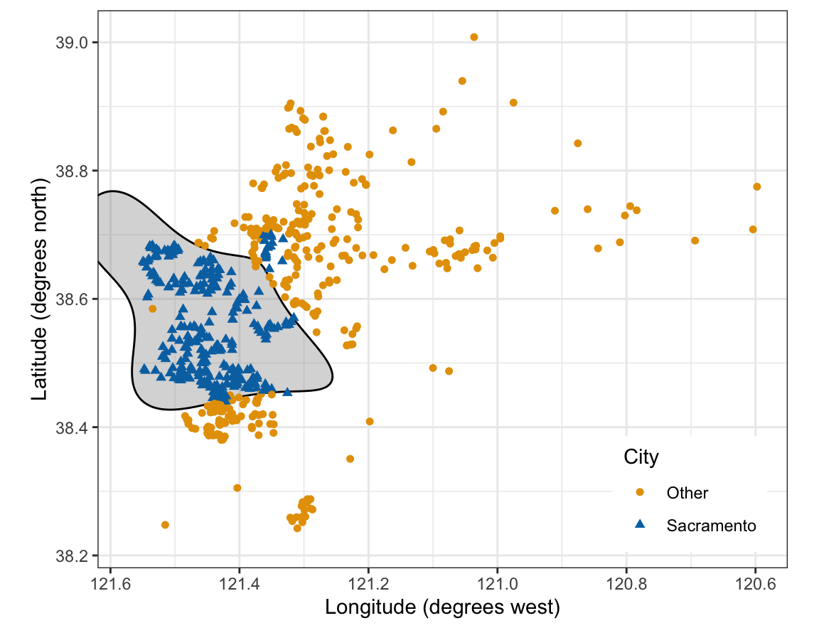
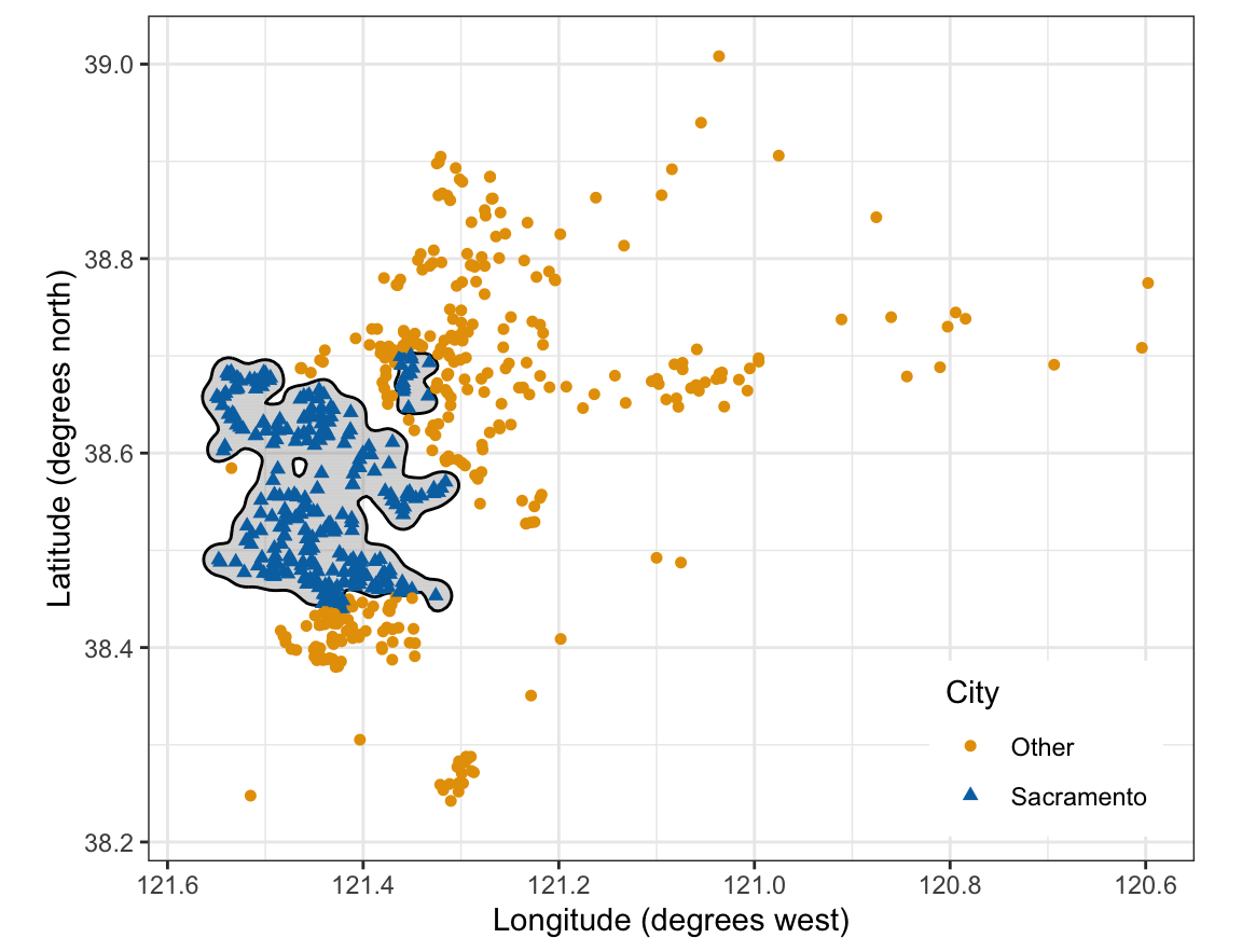
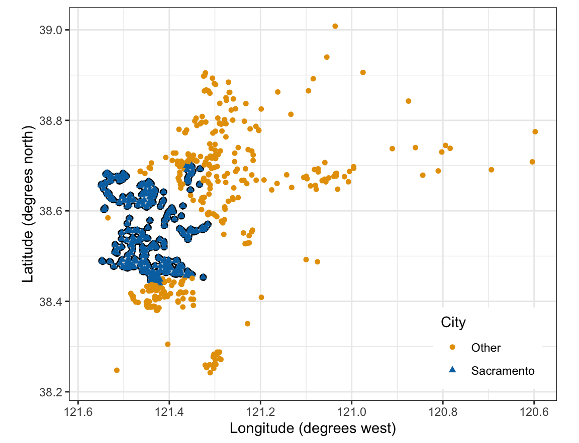
- Radial kernel: 1 when \(x = x_i\), falling toward 0 as \(x\) moves away: local
- \(K = 0.01\) at distance \(\sqrt{\log(100)/\gamma}\) standard deviations
- Large \(\gamma\): small influence; small \(\gamma\): wide influence
Radial kernel: \(\gamma\), cost = 10
Fitting
Call:
svm(formula = place ~ longitude + latitude, data = train, kernel = "radial",
    cost = 1, gamma = 1)


Parameters:
   SVM-Type:  C-classification
 SVM-Kernel:  radial
       cost:  1

Number of Support Vectors: 147Tuning
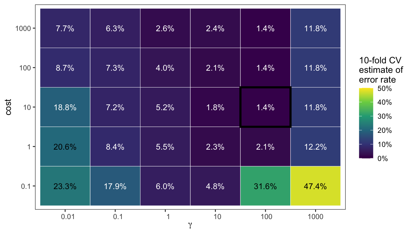
Grid
   cost gamma
23 10 100Grid: CV estimates
Test error
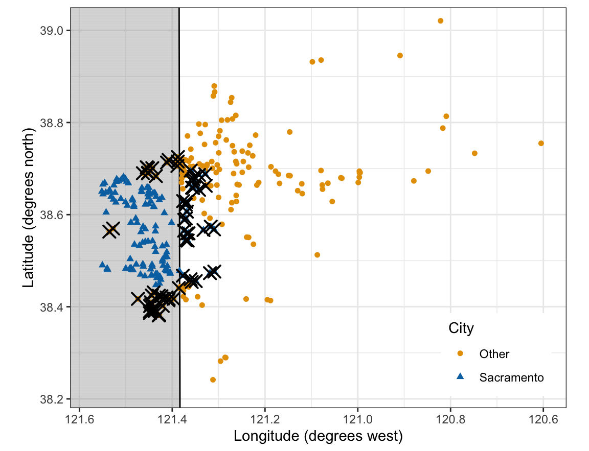
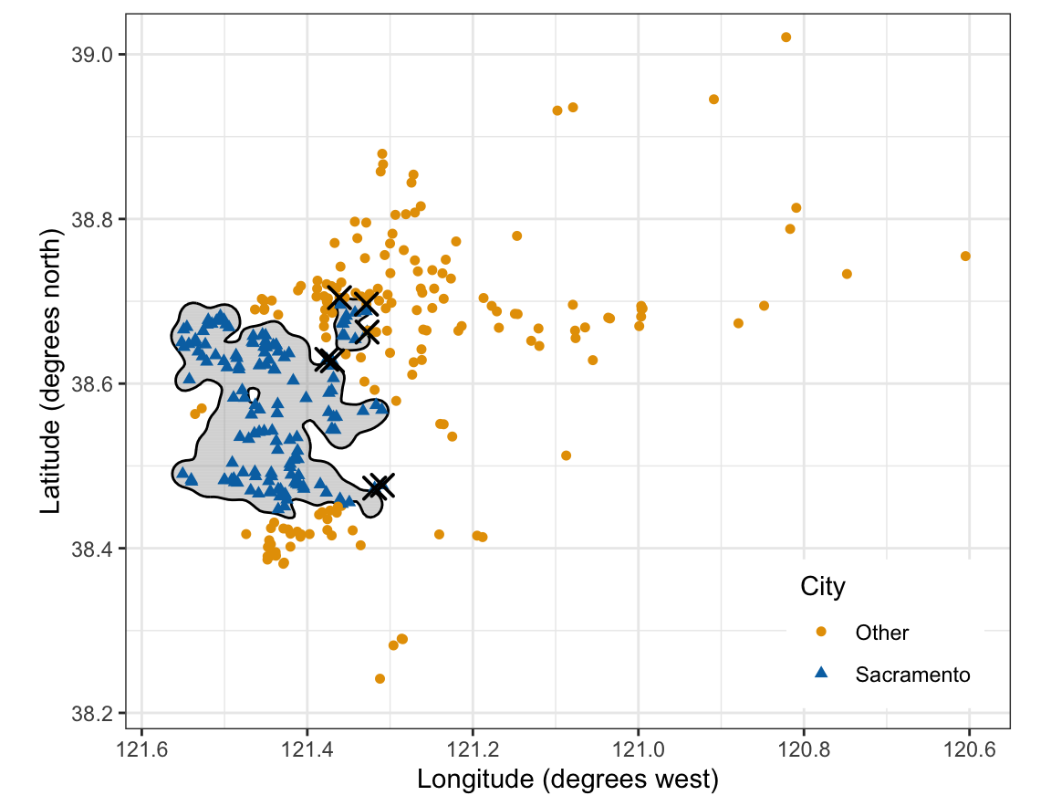
Test error: confusion matrices
$radial
            Predicted
Truth        Other Sacramento
  Other        165          2
  Sacramento     5        139

$linear
            Predicted
Truth        Other Sacramento
  Other        129         38
Sacramento 32 112- Test error rate: radial 2.3%, linear 22.5%
- Classifying every test home
Other: 46.3%
More than two classes
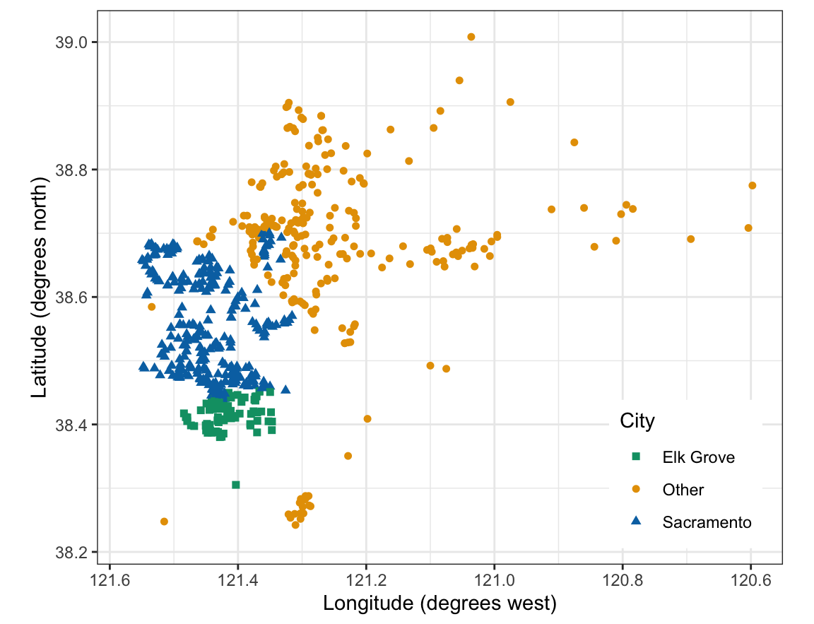
More than two classes
One versus one and one versus all
\(K\) classes, \(K > 2\):
- One versus one: a classifier for each of the \(\binom{K}{2}\) pairs of classes; the most votes wins
- One versus all: \(K\) classifiers, class \(k\) against all the others; the class with the largest \(\widehat{f}_k\left(x^*\right)\)
Pairwise voting
svm(): one versus one whenever the class has more than two levels- Confusion matrix of the test homes, three classes:
Elk Grove,Other,Sacramento
            Predicted
Truth        Elk Grove Other Sacramento
  Elk Grove         34     0          0
  Other              0   131          2
Sacramento 0 5 139- Test error rate: 2.3%
Hinge and logistic loss
Loss plus penalty
Support vector classifier, without slack variables:
\[ \underset{w_0, w}{\text{minimize}} \quad \sum_{i=1}^n \max\left[0, 1 - y_i f(x_i)\right] + \lambda\sum_{j=1}^p w_j^2, \qquad \lambda = \frac{1}{2\,\texttt{cost}}, \]
- \(f(x_i) = w_0 + w^\top x_i\) — fit, with \(w = (w_1, \ldots, w_p)^\top\)
- \(y_i = \pm 1\) — class of observation \(i\); \(n\) observations, \(p\) explanatory variables
- \(\max\left[0, 1 - y_if(x_i)\right]\) — hinge loss of observation \(i\)
- \(\lambda \ge 0\) — ridge penalty’s tuning parameter
Logistic loss
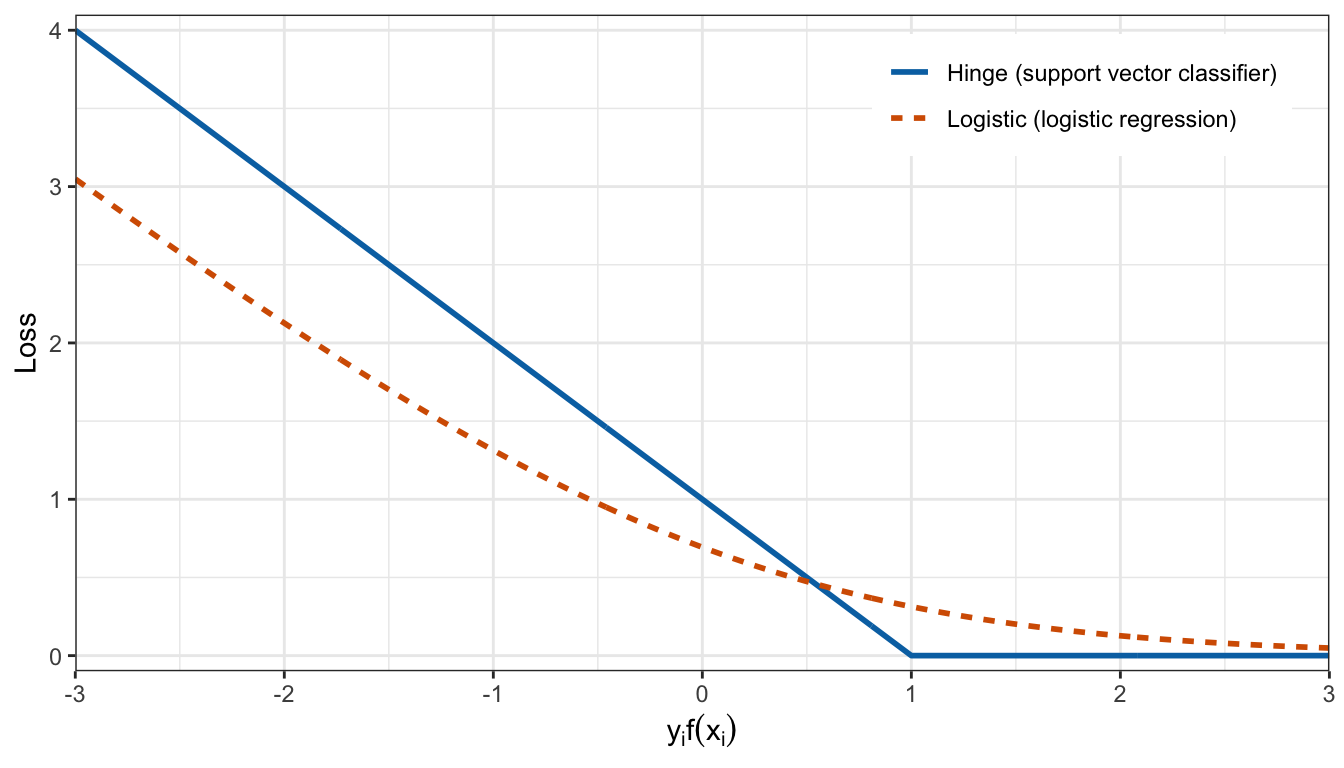
Logistic regression, negative log-likelihood:
\[ \sum_{i=1}^n \log\left(1 + e^{-y_i f(x_i)}\right). \]
Comparison
# Logistic regression on longitude and latitude, classified at 0.5.
logistic_fit <- glm(place ~ longitude + latitude, data = train,
                    family = binomial)
p_test <- predict(logistic_fit, test, type = "response")
logistic_class <- if_else(p_test > 0.5, "Sacramento", "Other")
mean(logistic_class != test$place)
[1] 0.221865- Logistic regression test error rate: 22.2%; linear support vector classifier: 22.5%
- The two classify 99.0% of the test homes the same way
- Logistic regression gives each test home a probability; the support vector classifier does not
Conclusion
- Polynomial features curve the boundary, but they are too many
- A new observation is classified through inner products with the support vectors
- A kernel replaces the inner product: linear, polynomial, radial
- The radial kernel is local; \(\gamma\) trades bias against variance
costand \(\gamma\) by cross-validation; judged by the test error rate- Hinge loss is zero outside the margin; logistic loss never is
DS 3030