2 Regression

Learning objectives

After this lecture you should be able to

identify a regression problem by its response variable, and write the model $Y_i = f(X_i) + \epsilon_i$ with its assumptions on $\epsilon_i$,
distinguish prediction from understanding as the goal of an analysis, and explain what each goal is willing to sacrifice,
define training MSE and test MSE, and explain why the training MSE is the wrong quantity to minimize,
interpret the U-shaped relationship between model flexibility and test MSE, and
state the bias-variance decomposition of the expected test MSE and identify which of its three terms no model can reduce.

2.1 Response variables

For regression models, our response variable is quantitative, continuous values.

For example,

Salary
Yield
Score
Concentration

2.2 True Model

The non-linear regression model of interest is

\[Y_i = f(X_i) + \epsilon_i\] where, for observation $i$,

$Y_i$ is the response variable,
$X_i = (X_{i1},\ldots,X_{ip})$ is the collection of explanatory variables, and
$\epsilon_i$ is the error with $E[\epsilon_i] = 0$, $Var[\epsilon_i] = \sigma^2$, and independent of $X_i$.

2.2.1 Goal

Based on data $(x_i, y_i)$ for $i=1,\ldots,n$, obtain an estimate of the function, $\hat{f}()$.

2.3 Prediction vs Understanding

Prediction: we don’t care about interpretation, we just want the model that fits the best

Understanding: we would like the model to fit well, but are willing to sacrifice some fit to have a model that is simple to understand

Examples

Compared to a high school diploma, having a bachelor’s degree increases starting salary by $20,000.
A master’s degree in data science typically yields a 5% to 25% salary increase compared to a bachelor’s degree.
After adjusting for age, gender, and other factors, the average salary of a data scientist is $X higher than that of a software engineer.

2.4 Model Evaluation

When prediction is the goal, we evaluate the model through its mean squared error:

\[\text{Training MSE} = \frac{1}{n} \sum_{i=1}^n (y_i - \hat{y}_i)^2 = \frac{1}{n} \sum_{i=1}^n \left[y_i - \hat{f}(x_i)\right]^2\] as written, this is the training MSE since we used the same data to estimate $\hat{f}$ as we used to compute the MSE.

We are actually more interested in how well our model fits test data, i.e. data that were not used to estimate $\hat{f}$. Thus, we typically estimate the expected test MSE:

\[\text{Test MSE} = E\left\{\left[Y - \hat{f}(X)\right]^2\right\}\approx \frac{1}{m} \sum_{i=1}^m \left[\tilde{y}_i - \hat{f}(\tilde{x}_i)\right]^2\] and we refer to this simply as the test MSE.

2.5 Bias-variance Tradeoff

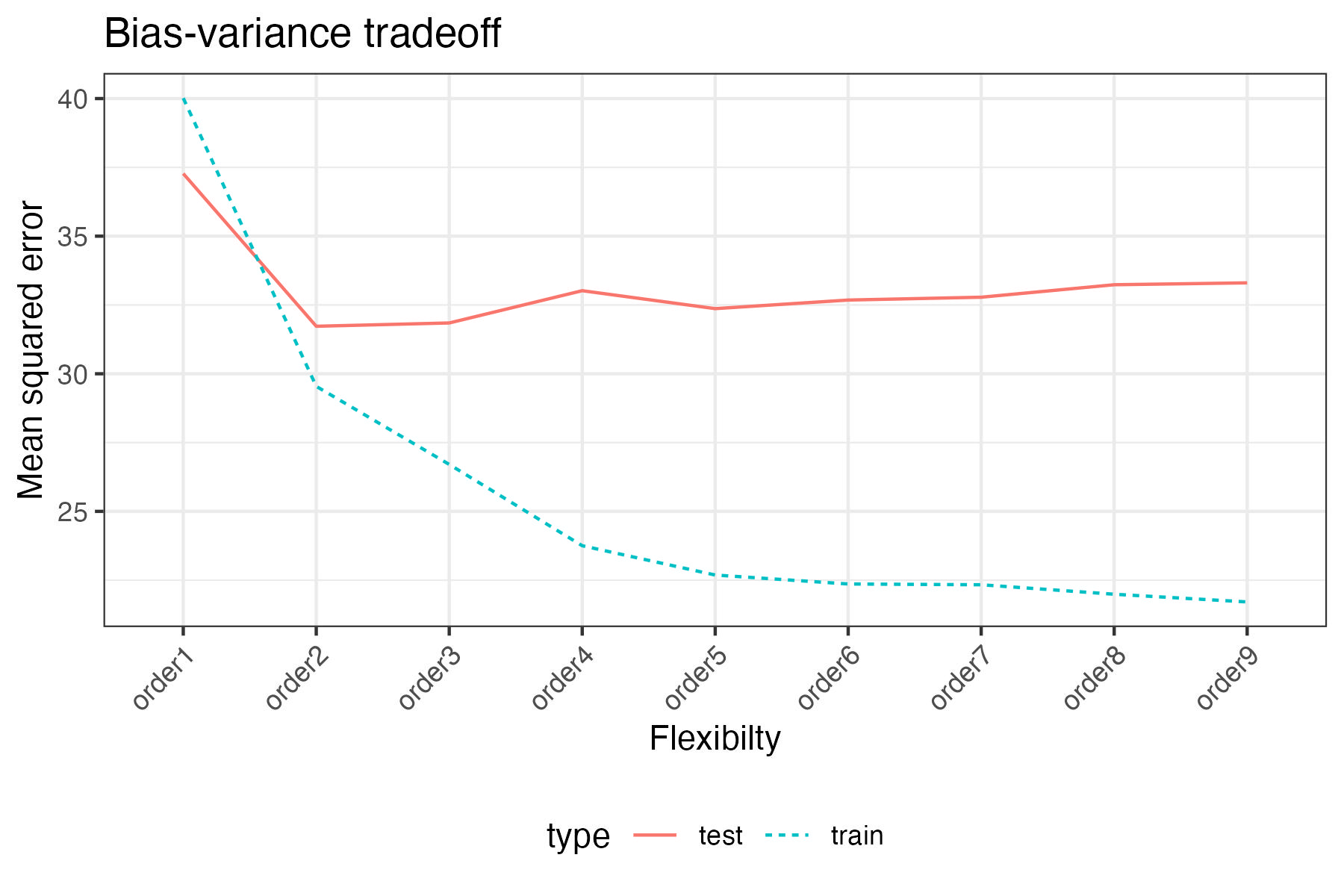
Using this Regression script, we create this plot that has the model flexibility on the x-axis and the test MSE on the y-axis.

2.6 Bias-variance Tradeoff (Mathematically)

Over different training data sets, we want to reduce the expected test MSE, which can be decomposed as follows:

\[E\left[\left(Y-\hat{f}(X)\right)^2\right] = Var\left[\hat{f}(X)\right] + Bias\left[\hat{f}(X)\right]^2 + Var[\epsilon]\] where

$Var[\hat{f}(X)]$ is the variance
$Bias[\hat{f}(X)]$ is the bias
$Var[\epsilon]$ is the irreducible error