x <- 1:10
y <- as.numeric(x > 5)
toy <- tibble(x = x, y = y, class = factor(y))12 Problems in Logistic Regression
TipLearning objectives
After this lecture you should be able to
- define complete and quasi-complete separation as conditions on the data, stated through the existence of a coefficient vector whose linear predictor classifies every observation correctly,
- derive, from the Bernoulli log-likelihood, why separation leaves \(\ell\) with a supremum but no finite maximizer,
- diagnose an enormous coefficient paired with a still larger standard error, alongside a
glm.fitwarning, as separation rather than as evidence about the feature, - evaluate the responses available when separation occurs — a larger sample, a simpler model, or a fit still usable for prediction away from the separated region — and distinguish separation from a warning that a single extreme observation caused, and
- state linear and logistic regression as distributional statements, identify the independence, normality, linearity, and constant-variance assumptions embedded in each, distinguish which of those carry over to logistic regression and which do not, and compare the potential problems of linear regression against their logistic regression counterparts to determine which do not transfer.
12.1 Separation
Every logistic regression in the previous three lectures converged, returned standard errors of a believable size, and produced \(z\)-statistics that could be read against a normal distribution. Nothing in those outputs suggested that maximum likelihood might do anything else.
It can. Least squares always returns an estimate as long as \(\mathbf{X}^\top \mathbf{X}\) is invertible, because \(\hat\beta = (\mathbf{X}^\top \mathbf{X})^{-1}\mathbf{X}^\top y\) is a formula. Maximum likelihood for logistic regression has no formula: \(\hat\beta\) is defined as the maximizer of \(\ell(\beta)\), and a function need not have one.
So ask what happens at the opposite extreme from a useless feature: one that predicts the response perfectly.
12.1.1 Perfectly predictive feature
Question. Suppose a single feature sorts the two classes without a single mistake. What does glm() estimate?
Data. Ten observations, constructed rather than collected, because the point is about a data-generating arrangement rather than about any real measurement:
- \(x_i\) takes the values \(1, 2, \ldots, 10\), and
- \(y_i = 1\) exactly when \(x_i > 5\), so the five smallest feature values carry \(y = 0\) and the five largest carry \(y = 1\).
NoteCode
toy_eda_plot <- ggplot(toy, aes(x = x, y = y, color = class, shape = class)) +
  geom_vline(xintercept = 5.5, linetype = "dashed", color = "grey50") +
  geom_point(size = 3) +
  scale_x_continuous(breaks = x) +
  scale_y_continuous(breaks = c(0, 1)) +
  scale_color_manual(values = c("#0072B2", "#D55E00")) +
  labs(x = "x", y = "y", color = "y", shape = "y",
       title = "A perfectly predictive feature")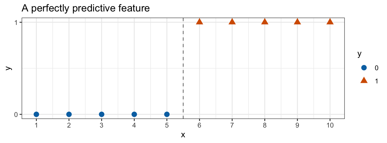
Every \(y = 0\) lies to the left of the dashed line and every \(y = 1\) lies to the right, with a gap of one unit between the last \(0\) and the first \(1\). No observation contradicts the rule “predict \(1\) when \(x > 5.5\),” and the dashed line could be moved anywhere in \((5, 6)\) without changing that.
Now fit the model.
toy_glm <- glm(y ~ x, data = toy, family = "binomial")Warning: glm.fit: algorithm did not convergeWarning: glm.fit: fitted probabilities numerically 0 or 1 occurredsummary(toy_glm)
Call:
glm(formula = y ~ x, family = "binomial", data = toy)

Coefficients:
            Estimate Std. Error z value Pr(>|z|)
(Intercept)   -245.8   337834.2  -0.001    0.999
x               44.7    61172.1   0.001    0.999

(Dispersion parameter for binomial family taken to be 1)

    Null deviance: 1.3863e+01  on 9  degrees of freedom
Residual deviance: 7.8648e-10  on 8  degrees of freedom
AIC: 4

Number of Fisher Scoring iterations: 25
The two warnings are the output of the chunk above, not a defect in it. This lecture is about the condition that produces them, so they are left visible here and in both examples that follow rather than suppressed; recognizing the exact strings glm.fit: algorithm did not converge and glm.fit: fitted probabilities numerically 0 or 1 occurred is part of what is being taught.
NoteCode
toy_coef <- summary(toy_glm)$coefficients
toy_b    <- toy_coef[, "Estimate"]
toy_se   <- toy_coef[, "Std. Error"]
toy_z    <- toy_coef[, "z value"]
toy_p    <- toy_coef[, "Pr(>|z|)"]
toy_ratio <- toy_se / abs(toy_b)
Read the coefficient table one column at a time.
- The estimates are \(\hat\beta_0 = -245.8\) and \(\hat\beta_1 = 44.7\). A slope of \(44.7\) log-odds per unit of \(x\) is an odds ratio of \(e^{44.7}\), a number with 20 digits before the decimal point.
- The standard errors are larger still: 337,834 and 61,172, each roughly 1,400 times the coefficient it belongs to.
- So \(z = 0.001\) for the slope, with a \(p\)-value of \(0.999\). The feature that predicts the response without error is not statistically significant.
Two more lines of the output say the same thing in different ways. The number of Fisher scoring iterations is 25, which is glm()’s default maximum, so the algorithm stopped because it ran out of iterations rather than because it arrived anywhere, and toy_glm$converged is FALSE. The residual deviance is \(7.9 \times 10^{-10}\), which is \(-2\ell(\hat\beta)\): the log-likelihood at the reported estimates is zero to within rounding, meaning the model reproduces all 10 observed responses exactly.
A model that fits the training data perfectly and reports no significant coefficient is not a contradiction. It is the signature of separation.
12.1.2 Complete and quasi-complete separation
Separation is defined through the linear predictor rather than through a picture.
Write \(x_i\) for the \(i\)th row of the model matrix and \(b\) for a candidate coefficient vector, so \(x_i b\) is the linear predictor that \(b\) assigns to observation \(i\). The data exhibit complete separation (also called perfect separation) if there exists a \(b\) with
\[x_i b > 0 \ \text{ for every } i \text{ with } y_i = 1, \qquad x_i b < 0 \ \text{ for every } i \text{ with } y_i = 0,\]
where
- \(x_i = (1, x_{i1}, \ldots, x_{ip})\) is the feature row for observation \(i\),
- \(b\) is any vector in \(\mathbb{R}^{p+1}\), not necessarily the maximum likelihood estimate, and
- \(y_i \in \{0, 1\}\) is the observed response.
Note that this is a condition on the data, not on a fitted model: it asks whether some \(b\) works, and says nothing about \(\hat\beta\), which under this condition does not exist. Since the probability that \(b\) implies exceeds \(0.5\) exactly when \(x_i b > 0\), the condition says the decision boundary of the previous lecture, drawn using \(b\), classifies every training observation correctly, with no observation lying on the boundary itself.
The data exhibit quasi-complete separation if the strict inequalities can be weakened to
\[x_i b \ge 0 \ \text{ for every } i \text{ with } y_i = 1, \qquad x_i b \le 0 \ \text{ for every } i \text{ with } y_i = 0,\]
for some \(b \ne 0\), with equality holding for at least one observation. Some observations sit exactly on the boundary; none sits on the wrong side of it.
Both conditions break maximum likelihood, and neither is visible in a coefficient table without knowing what to look for.
In the single-feature examples that follow, \(x_i\) reverts to naming the scalar feature value rather than the row of \(\mathbf{X}\), exactly as it did in the opening toy example above.
12.1.3 Tied feature values
Question. The toy data above are completely separated, and glm() announced the trouble with a convergence warning. Does a quasi-complete separation announce itself the same way?
Data. Ten observations again, with one tie: two of them share a feature value and carry opposite responses, and everything else is arranged as before.
xq <- c(1, 2, 3, 4, 5, 5, 6, 7, 8, 9)
yq <- c(0, 0, 0, 0, 0, 1, 1, 1, 1, 1)
quasi <- tibble(xq = xq, yq = yq, class = factor(yq))- \(x_i\) takes the values \(1, 2, 3, 4, 5, 5, 6, 7, 8, 9\), with the value \(5\) recorded twice, and
- \(y_i = 0\) for the first five rows and \(y_i = 1\) for the last five, so the two observations at \(x = 5\) carry opposite responses.
NoteCode
quasi_eda_plot <- ggplot(quasi, aes(x = xq, y = yq,
                                    color = class, shape = class)) +
  geom_vline(xintercept = 5, linetype = "dashed", color = "grey50") +
  geom_point(size = 3) +
  scale_x_continuous(breaks = sort(unique(xq))) +
  scale_y_continuous(breaks = c(0, 1)) +
  scale_color_manual(values = c("#0072B2", "#D55E00")) +
  labs(x = "x", y = "y", color = "y", shape = "y",
       title = "A tie on the boundary")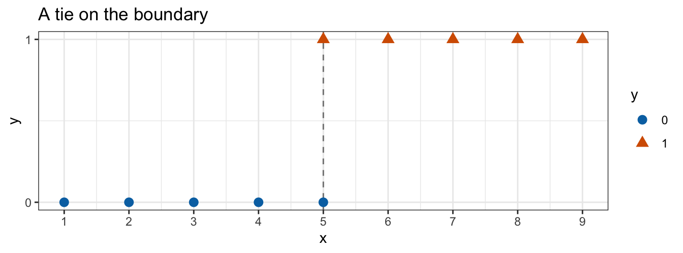
The dashed line now passes through two observations rather than between the classes: one \(y = 0\) and one \(y = 1\) sit on it. Every other observation is on the side its response requires, but there is no gap left to move the line into.
One tie is enough to turn complete separation into quasi-complete. Complete separation needs a gap between the classes; quasi-complete separation does not, needing only that no observation falls strictly on the wrong side. Take \(b = (-5\beta_1, \beta_1)\) for any \(\beta_1 > 0\): the two observations at \(x = 5\) get a linear predictor of \(\beta_1(5 - 5) = 0\), every observation with \(x_i > 5\) gets \(x_i b > 0\), and every observation with \(x_i < 5\) gets \(x_i b < 0\). The weak inequalities hold for all ten observations and the strict ones fail for two, which is exactly quasi-complete separation.
Now fit the model.
quasi_glm <- glm(yq ~ xq, data = quasi, family = "binomial")Warning: glm.fit: fitted probabilities numerically 0 or 1 occurredsummary(quasi_glm)
Call:
glm(formula = yq ~ xq, family = "binomial", data = quasi)

Coefficients:
            Estimate Std. Error z value Pr(>|z|)
(Intercept)   -98.16   39288.59  -0.002    0.998
xq             19.63    7857.72   0.002    0.998

(Dispersion parameter for binomial family taken to be 1)

    Null deviance: 13.8629  on 9  degrees of freedom
Residual deviance:  2.7726  on 8  degrees of freedom
AIC: 6.7726

Number of Fisher Scoring iterations: 21
The single warning is the point of this example. The completely separated fit above raised two — glm.fit: algorithm did not converge and glm.fit: fitted probabilities numerically 0 or 1 occurred — and this fit raises only the second. The warning that most nearly settles a diagnosis of separation is the one that does not fire here.
NoteCode
quasi_coef  <- summary(quasi_glm)$coefficients
quasi_b     <- quasi_coef[, "Estimate"]
quasi_se    <- quasi_coef[, "Std. Error"]
quasi_z     <- quasi_coef[, "z value"]
quasi_p     <- quasi_coef[, "Pr(>|z|)"]
quasi_ratio <- quasi_b[1] / quasi_b[2]
The estimates are as unusable as in the completely separated case: \(\hat\beta_1 = 19.63\) with a standard error of 7,858, giving \(z = 0.002\) and a \(p\)-value of \(0.998\). The intercept is \(\hat\beta_0 = -98.16\), and \(\hat\beta_0 / \hat\beta_1 = -5\) to machine precision: the iteration is walking out along the family \(b = (-5\beta_1, \beta_1)\) derived above and stopping at an arbitrary point on it.
What the fit reports about itself reads differently from the toy fit, though. The number of Fisher scoring iterations is 21, short of glm()’s default maximum of 25, and quasi_glm$converged is TRUE. A reported convergence is not evidence that an estimate is trustworthy.
The residual deviance is 2.7726 rather than essentially zero, and the two tied observations are why. As \(\beta_1\) grows the fitted probability at \(x = 5\) stays at \(\text{logistic}(0) = 0.5\), so those two observations contribute
\[-2\left[\log(0.5) + \log(0.5)\right] = 2.7726\]
to the deviance no matter how large \(\beta_1\) becomes, while every other observation’s contribution goes to zero. Under complete separation the deviance falls to zero; under quasi-complete separation it falls to whatever the boundary ties contribute.
12.1.4 Maximum likelihood failure
The simple logistic regression lecture derived the Bernoulli log-likelihood
\[\ell(\beta_0, \beta_1) = \sum_{i=1}^n \left\{ y_i (\beta_0 + \beta_1 x_i) - \log\left(1 + e^{\beta_0 + \beta_1 x_i}\right) \right\},\]
and nothing beyond that is needed to see what goes wrong.
Restrict attention to a one-parameter family of coefficient vectors that all place the decision boundary at \(x = 5.5\), by setting \(\beta_0 = -5.5\beta_1\). Then the linear predictor is \(\eta_i = \beta_1(x_i - 5.5)\) and
\[\ell(\beta_1) = \sum_{i=1}^n \left\{ y_i \beta_1 (x_i - 5.5) - \log\left(1 + e^{\beta_1(x_i - 5.5)}\right) \right\},\]
where
- \(\beta_1\) is the only free parameter, and
- \(p_i = \text{logistic}(\beta_1(x_i - 5.5))\) is the probability the family implies for observation \(i\).
Differentiating with respect to \(\beta_1\), by the same steps that produced the score equations,
\[\frac{d\ell}{d\beta_1} = \sum_{i=1}^n (x_i - 5.5)\left(y_i - p_i\right).\]
Now use the separation. Every observation with \(y_i = 1\) has \(x_i > 5.5\), so \(x_i - 5.5 > 0\), and \(y_i - p_i = 1 - p_i > 0\) because \(p_i < 1\) always. Every observation with \(y_i = 0\) has \(x_i < 5.5\), so \(x_i - 5.5 < 0\), and \(y_i - p_i = -p_i < 0\). Both cases contribute a positive product, so
\[\frac{d\ell}{d\beta_1} > 0 \quad \text{for every finite } \beta_1.\]
The derivative is never zero, so there is no stationary point and no finite maximizer. Meanwhile \(\ell < 0\) for every finite \(\beta_1\), and as \(\beta_1 \to \infty\) each \(p_i\) approaches the \(y_i\) it is paired with, so every term approaches \(\log 1 = 0\) and \(\ell \to 0\). The log-likelihood has a supremum of \(0\) that it attains only in the limit.
What glm() reports is therefore not an estimate. It is whatever point the iteration happened to be at when it stopped, and the reported standard errors come from the curvature of \(\ell\) at that point — curvature that is flattening toward zero as the iteration runs, which is why they grow without bound.
Drawing the fitted curve at a few values of \(\beta_1\) along this family shows what the derivative is describing.
NoteCode
toy_curve_betas <- c(0.5, 1, 2, 5)

toy_curves <- expand_grid(beta1 = toy_curve_betas,
                          xg = seq(0, 11, length.out = 400)) |>
  mutate(p = plogis(beta1 * (xg - 5.5)),
         beta1 = factor(sprintf("beta[1] == %.1f", beta1),
                        levels = sprintf("beta[1] == %.1f", toy_curve_betas)))

toy_curve_plot <- ggplot(toy_curves,
                         aes(x = xg, y = p, color = beta1, linetype = beta1)) +
  geom_line(linewidth = 0.9) +
  geom_point(data = toy, aes(x = x, y = y), inherit.aes = FALSE,
             size = 2, alpha = 0.7) +
  scale_color_manual(values = c("#E69F00", "#56B4E9", "#009E73", "#CC79A7"),
                     labels = scales::parse_format()) +
  scale_linetype_manual(values = c("solid", "dashed", "dotted", "dotdash"),
                        labels = scales::parse_format()) +
  scale_y_continuous(breaks = c(0, 0.5, 1)) +
  labs(x = "x", y = "p(x)", color = NULL, linetype = NULL,
       title = "Fitted curves along the family with boundary fixed at 5.5")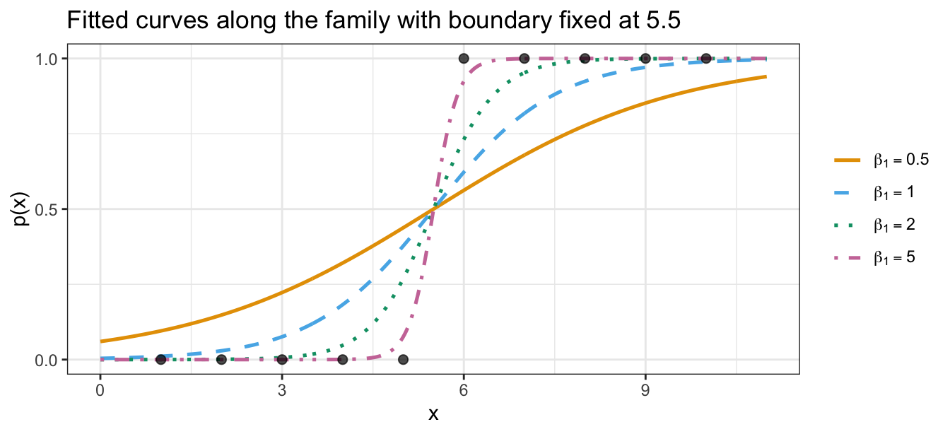
Each increase in \(\beta_1\) steepens the curve at the boundary and pushes it closer to \(0\) on the left and to \(1\) on the right, so every fitted probability moves toward the response it is paired with. Nothing stops this: the curve approaches a step function and the likelihood approaches \(1\).
Evaluating \(\ell\) along the same family puts numbers on it.
NoteCode
toy_loglik <- function(beta1) {
  eta <- beta1 * (toy$x - 5.5)
  sum(toy$y * eta - log(1 + exp(eta)))
}

toy_ll_table <- tibble(beta1 = c(0, 0.5, 1, 2, 5, 8)) |>
  mutate(ll = map_dbl(beta1, toy_loglik),
         L  = exp(ll)) |>
  mutate(beta1 = sprintf("%.1f", beta1),
         ll    = sprintf("%.3f", ll),
         L     = sprintf("%.3f", L)) |>
  knitr::kable(col.names = c("$\\beta_1$", "$\\ell(\\beta_1)$",
                             "$L(\\beta_1)$"),
               align = "ccc")

toy_ll_curve <- tibble(beta1 = seq(0, 8, length.out = 400)) |>
  mutate(ll = map_dbl(beta1, toy_loglik))

toy_ll_plot <- ggplot(toy_ll_curve, aes(x = beta1, y = ll)) +
  geom_hline(yintercept = 0, linetype = "dashed", color = "grey50") +
  geom_line(color = "#0072B2", linewidth = 0.9) +
  labs(x = expression(beta[1]), y = "Log-likelihood",
       title = expression(paste("Log-likelihood along the family ",
beta[0] == -5.5 * beta[1])))| \(\beta_1\) | \(\ell(\beta_1)\) | \(L(\beta_1)\) |
|---|---|---|
| 0.0 | -6.931 | 0.001 |
| 0.5 | -2.950 | 0.052 |
| 1.0 | -1.590 | 0.204 |
| 2.0 | -0.739 | 0.477 |
| 5.0 | -0.159 | 0.853 |
| 8.0 | -0.036 | 0.964 |
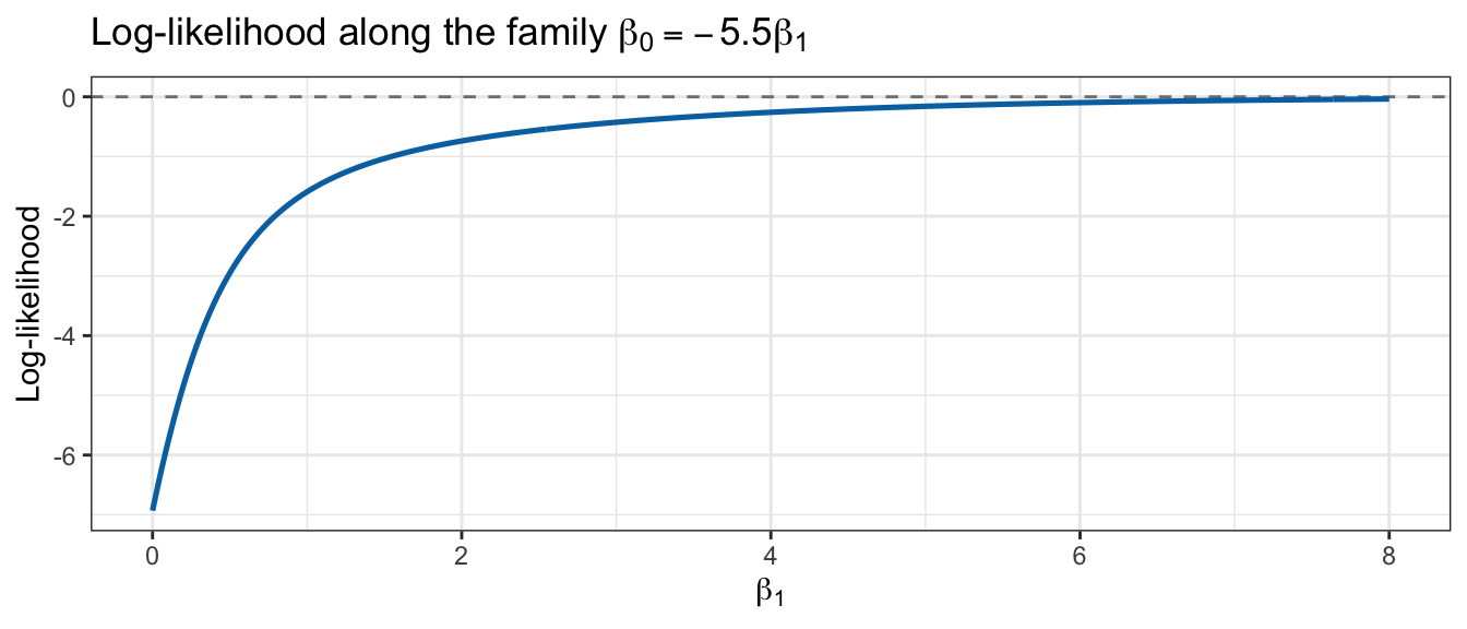
The log-likelihood rises steeply at first and then flattens against the dashed line at \(0\) without ever touching it, exactly as the derivative predicted. The likelihood column reaches 0.964 at \(\beta_1 = 8\) and would keep climbing toward \(1\) for larger values.
NoteBeyond this course
Two numerical artifacts surface when \(\ell\) is evaluated by hand at large \(\beta_1\). Neither changes any conclusion above, and neither is tested here.
toy_loglik_prob <- function(beta1) {
  p <- plogis(beta1 * (toy$x - 5.5))
  sum(toy$y * log(p) + (1 - toy$y) * log(1 - p))
}

artifact_grid <- seq(0.1, 400, by = 0.1)
first_nan <- artifact_grid[which(is.na(map_dbl(artifact_grid,
                                               toy_loglik_prob)))[1]]
first_inf <- artifact_grid[which(is.infinite(map_dbl(artifact_grid,
                                                     toy_loglik)))[1]]
Evaluating \(\ell\) on the probability scale as \(\sum_i \{y_i \log p_i + (1 - y_i)\log(1 - p_i)\}\) is algebraically identical to the form used above, but in this example it returns NaN from \(\beta_1 = 8.2\) onward. Once \(p_i\) rounds to exactly \(1\), the term \((1 - y_i)\log(1 - p_i)\) becomes \(0 \times \log 0 = 0 \times (-\infty)\), which is NaN.
The \(\eta\)-scale form survives further but eventually fails too: at \(\beta_1 = 157.8\) the largest \(e^{\eta_i}\) overflows to Inf, and \(\ell\) returns \(-\infty\).
Neither is a property of \(\ell\), which is finite, negative, and increasing at every one of those values. Both are finite-precision arithmetic running out of room, which is also the mechanism behind the fitted probabilities numerically 0 or 1 warning. The range \(0 \le \beta_1 \le 8\) plotted above stays clear of both.
12.2 Muscular dystrophy carrier screening
Constructed data makes the mechanism visible, and it also makes separation look unmistakable. It is not always. Real data can trigger the same warning without being separated at all, and telling the two cases apart takes one more step after the warning appears.
Question. Duchenne muscular dystrophy is inherited through female carriers, who show no symptoms themselves. Can a blood test identify likely carriers, so that a woman with a family history can be counseled about her risk?
Data. Sleuth3::ex2012 records 120 women, each already classified by other means:
Group:Casefor a known carrier,Controlotherwise. There are 38 carriers and 82 non-carriers. This is the response, with \(Y_i = 1\) for a carrier.CK: serum creatine kinase, an enzyme that leaks from damaged muscle. This is the feature.H: serum hemopexin, a second blood measurement, recorded but not used below.
Case is the first level of Group, and glm() models the probability of a factor’s second level, so the event has to be set explicitly:
dmd <- Sleuth3::ex2012 |>
  mutate(Group = relevel(Group, ref = "Control"),
         case01 = as.numeric(Group == "Case"))
levels(dmd$Group)
[1] "Control" "Case"
NoteCode
# The jitter is computed once and stored, rather than left to geom_jitter(),
# so re-rendering does not move the points.
set.seed(20260919)
dmd <- dmd |> mutate(case_jittered = case01 + runif(n(), -0.04, 0.04))

max_control_ck <- max(dmd$CK[dmd$Group == "Control"])
n_above        <- sum(dmd$CK > max_control_ck)
n_case_below   <- sum(dmd$Group == "Case" & dmd$CK <= max_control_ck)

dmd_eda_plot <- ggplot(dmd, aes(x = CK, y = case_jittered,
                                color = Group, shape = Group)) +
  geom_vline(xintercept = max_control_ck, linetype = "dashed",
             color = "grey50") +
  geom_point(size = 1.8, alpha = 0.8) +
  scale_y_continuous(breaks = c(0, 1),
                     labels = c("Control (0)", "Case (1)")) +
  scale_color_manual(values = c("#0072B2", "#D55E00")) +
  labs(x = "Serum creatine kinase (CK)", y = "Carrier status",
       title = "Sleuth3::ex2012")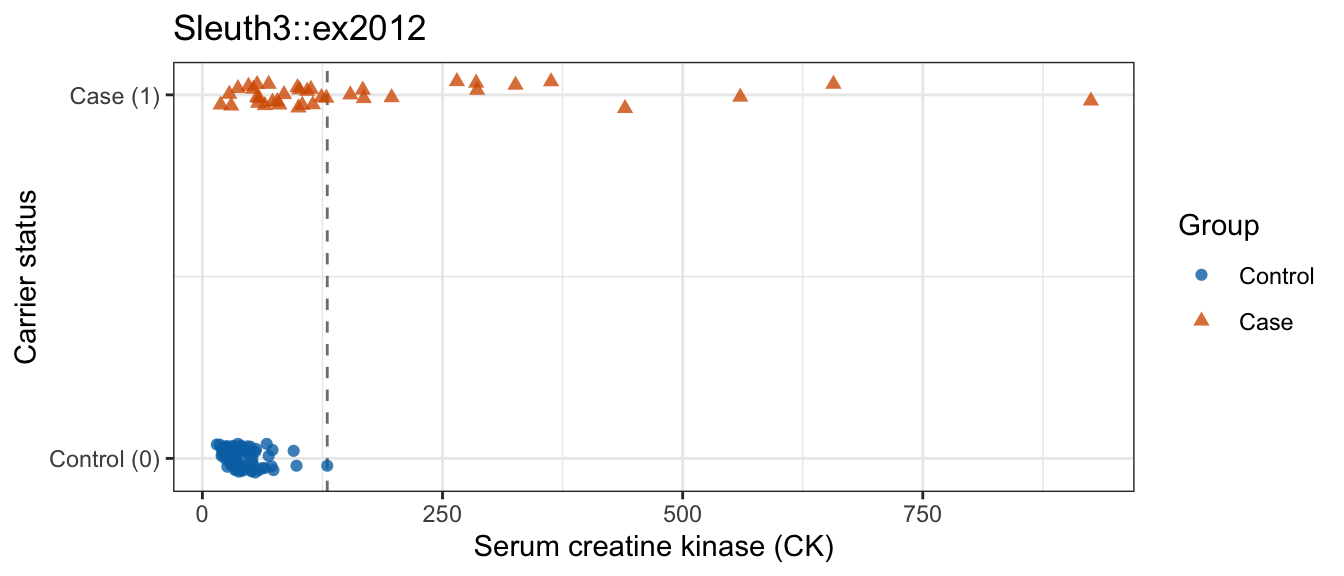
The dashed line marks 130, the largest CK recorded on any non-carrier. All 13 observations to its right are carriers. To its left the two groups overlap heavily: 25 of the 38 carriers have CK values in the same range as the non-carriers. Carriers have a median CK of 102.5 against 35 for non-carriers. No threshold on CK classifies these women without error, so this is not separation under either definition above.
Fit the model anyway.
dmd_glm <- glm(Group ~ CK, data = dmd, family = "binomial")Warning: glm.fit: fitted probabilities numerically 0 or 1 occurredsummary(dmd_glm)$coefficients Estimate Std. Error z value Pr(>|z|)
(Intercept) -3.96219273 0.6719084 -5.896924 3.703413e-09
CK 0.05073407 0.0106958 4.743364 2.101984e-06The warning from the toy example has reappeared. The convergence warning has not, and again this chunk’s warning is intended output rather than a defect.
NoteCode
dmd_b   <- coef(dmd_glm)
dmd_se  <- summary(dmd_glm)$coefficients[, "Std. Error"]
dmd_eta <- predict(dmd_glm)
dmd_p   <- fitted(dmd_glm)

dmd_or10    <- unname(exp(10 * dmd_b["CK"]))
dmd_ci10    <- exp(10 * confint.default(dmd_glm)["CK", ])
glm_eps     <- 10 * .Machine$double.eps
n_triggered <- sum(dmd_p > 1 - glm_eps | dmd_p < glm_eps)

# The true mathematical value of 1 - logistic(eta), computed without ever
# forming logistic(eta) itself, so it is not limited by how close to 1 a
# double can get.
true_gap <- exp(-max(dmd_eta)) / (1 + exp(-max(dmd_eta)))

dmd_tail_gaps <- (1 - dmd_p)[order(-dmd$CK)][1:5]

dmd_tail_table <- dmd |>
  mutate(eta = dmd_eta, p = dmd_p) |>
  slice_max(CK, n = 5) |>
  transmute(CK,
            Group = as.character(Group),
            eta = sprintf("%.1f", eta),
            gap = sprintf("$%s$", sci(1 - p))) |>
  knitr::kable(col.names = c("CK", "Group", "$\\hat\\eta$", "$1 - \\hat p$"),
               align = "ccrr")
The estimated slope is \(\hat\beta_1 = 0.0507\) with a standard error of 0.0107, a ratio of \(z = 4.74\). The algorithm reports dmd_glm$converged as TRUE after 7 iterations. Nothing in the coefficient table resembles the toy example’s standard error of 61,172.
What the warning is responding to sits at the far right of the plot. The last column below is \(1 - \hat p\) as fitted() reports it.
| CK | Group | \(\hat\eta\) | \(1 - \hat p\) |
|---|---|---|---|
| 925 | Case | 43.0 | \(2.2 \times 10^{-16}\) |
| 657 | Case | 29.4 | \(1.8 \times 10^{-13}\) |
| 560 | Case | 24.4 | \(2.4 \times 10^{-11}\) |
| 440 | Case | 18.4 | \(1.1 \times 10^{-8}\) |
| 363 | Case | 14.5 | \(5.3 \times 10^{-7}\) |
The largest linear predictor in the fit is \(\hat\eta = 42.97\). Mathematically,
\[1 - \text{logistic}(\hat\eta) = \frac{e^{-\hat\eta}}{1 + e^{-\hat\eta}} = 2.2 \times 10^{-19}\]
at that value — far below \(2^{-53} = 1.1 \times 10^{-16}\), the gap between \(1\) and the largest double-precision number below it (.Machine$double.eps \(= 2^{-52} = 2.2 \times 10^{-16}\) is the corresponding gap just above \(1\)). No double can hold a probability that close to \(1\): computed directly, \(1\) minus that gap rounds to exactly \(1\). A fitted probability of exactly \(0\) or \(1\) would make the deviance infinite for any observation whose response disagreed with it, and would give that observation zero weight in the next iteration, so glm() does not let it happen — it clamps the linear predictor before inverting the link, and fitted() never leaves \([2.2 \times 10^{-16},\ 1 - 2.2 \times 10^{-16}]\). The top row of the table is therefore the clamped value rather than the true one: 3 orders of magnitude larger than the true gap just derived, and 3 orders of magnitude smaller than the row beneath it in the table — the column only looks like it descends smoothly.
glm() warns whenever a fitted probability comes within \(2.2 \times 10^{-15}\) of \(0\) or \(1\), and here exactly 1 of the 120 observations does.
So the warning fired for a reason that has nothing to do with the estimator failing. One woman has a CK of 925, while the other 119 observations sit at 657 or below, and the fitted curve has saturated well before it reaches her.
Conclusion. Creatine kinase is strongly associated with carrier status: each additional 10 units of CK multiplies the estimated odds of being a carrier by 1.66 (95% CI 1.35 to 2.05). The estimate is finite, its standard error is small relative to it, and the iteration converged, so the warning here is a report about one extreme observation rather than about the estimator. The same warning in the toy example meant the estimate did not exist.
12.3 Separation diagnosis and response
The examples above give the same warning for different reasons, so the warning is where an investigation starts rather than where it ends. What settles the question is the coefficient table.
12.3.1 Recognizing separation
- A
glm.fit: algorithm did not convergewarning. This one is close to conclusive: when a strictly concave log-likelihood has a finite maximizer, the algorithm locates it in a handful of iterations. - A
glm.fit: fitted probabilities numerically 0 or 1 occurredwarning. This one is not conclusive on its own, as the muscular dystrophy example shows, but separation always produces it. - A coefficient whose magnitude is absurd on the feature’s own scale. An odds ratio of \(e^{44.7}\) per unit is not a quantity any real process produces.
- A standard error far larger than the coefficient it belongs to, so that a feature which classifies the training data perfectly returns \(z \approx 0\) and a \(p\)-value near \(1\). This is the diagnostic that is hardest to misread, because it is the reverse of what a strong feature normally looks like.
- Under complete separation, a residual deviance of essentially zero, meaning the fitted probabilities reproduce every observed response exactly. Under quasi-complete separation the deviance settles at whatever the tied observations on the boundary contribute, so it is small rather than zero.
- Fitted probabilities numerically indistinguishable from \(0\) or \(1\) in
fitted(), for observations on the separated side of the boundary. They are never exactly \(0\) or \(1\):glm()clamps them into \([2.2 \times 10^{-16},\ 1 - 2.2 \times 10^{-16}]\), so that is what a separated observation returns.
Comparing each \(|\hat\beta_j|\) against its standard error takes one line and settles the question; fit$converged is informative only when it is FALSE, since a quasi-complete separation can report convergence and still leave no usable estimate.
12.3.2 Available responses
Within the methods this course has covered, there are three responses.
Collect more data. Separation is a property of a sample, not of the population it came from. Ten observations and one threshold feature separate almost by construction; 120 observations with two overlapping distributions do not, even with one CK value 22 times the sample median. The probability that a sample happens to be separated falls as \(n\) grows and as the classes overlap more.
Simplify the model. If a feature or a dummy-coded level is what makes the data separable, and that feature is not the object of the analysis, dropping it or merging it with another level removes the separation. This is most common with a categorical feature that has a level in which the event never occurs: that level alone can separate the data, and combining it with a neighboring level fixes the fit without touching the rest of the model.
Use the fit for what it can still support. Separation destroys the coefficient, not necessarily the classification. The toy model’s slope is meaningless, but its decision boundary sits between \(x = 5\) and \(x = 6\) and classifies every observation correctly. A model that separates on one feature can still produce usable predicted classes away from the separated region, as long as no probability, odds ratio, standard error, or \(p\)-value involving the offending coefficient is reported.
NoteBeyond this course
The principled fix is to stop maximizing \(\ell(\beta)\) by itself and maximize a penalized version, \(\ell(\beta) - \lambda \cdot \text{pen}(\beta)\), where the penalty grows with the magnitude of \(\beta\). A penalty that increases without bound as \(\|\beta\| \to \infty\) restores a finite maximizer no matter how the data are arranged, because the penalty eventually outruns the gain in \(\ell\).
Firth’s penalized likelihood uses a penalty derived from the information matrix and is the standard remedy for separation; it also removes most of the small-sample bias in \(\hat\beta\). The ridge and lasso penalties forward-referenced in the multiple linear regression lecture do the same job from a different motivation, and both apply to logistic regression unchanged. A Bayesian analysis with a proper prior on \(\beta\) achieves the same effect again, since the prior plays the role of the penalty.
All of these are shrinkage methods, and shrinkage is ISLR2 Chapter 6 material. Name the fix if you meet separation before then; do not try to implement it from this callout.
12.4 Linear regression problems revisited
The flexibility lecture listed six potential problems for a linear regression: non-linearity, correlated errors, non-constant variance, outliers, high-leverage points, and collinearity. Separation has no counterpart on that list: whenever \(\mathbf{X}^\top \mathbf{X}\) is invertible, least squares evaluates a formula and so cannot fail this way. The six themselves transfer to logistic regression unevenly, and which of them transfer is settled by writing each model as a single distributional statement.
Linear regression is
\[Y_i \mid x_i \stackrel{ind}{\sim} N\left(x_i\beta, \sigma^2\right), \qquad i = 1, \ldots, n,\]
where
- \(Y_i\) is the response for observation \(i\),
- \(x_i = (1, x_{i1}, \ldots, x_{ip})\) is the \(i\)th row of the model matrix \(\mathbf{X}\), holding the intercept column and the \(p\) features,
- \(\beta = (\beta_0, \beta_1, \ldots, \beta_p)^\top\) is the coefficient vector, so that \(x_i\beta\) is the linear predictor for observation \(i\), and
- \(\sigma^2\) is the variance of the response around that linear predictor.
That one line carries four separate assumptions.
- Independence. The \(\mathrm{ind}\) over the \(\sim\) asserts that \(Y_1, \ldots, Y_n\) are independent of one another given the model matrix.
- Constant variance. \(Var[Y_i \mid x_i] = \sigma^2\), and \(\sigma^2\) carries no \(i\) subscript, so every observation has the same variance.
- Linearity. The mean is \(E[Y_i \mid x_i] = x_i\beta\), linear in the features.
- Normality. The response is normally distributed around its mean. This is the one assumption logistic regression does not keep in any form.
Logistic regression replaces the normal distribution with a Bernoulli one and the identity link with the logit:
\[Y_i \mid x_i \stackrel{ind}{\sim} \text{Bernoulli}\left(p(x_i)\right), \qquad \log\left[\frac{p(x_i)}{1 - p(x_i)}\right] = x_i\beta,\]
where
- \(p(x_i) = P(Y_i = 1 \mid x_i)\) is the probability of the event for observation \(i\).
The four assumptions come through the substitution unevenly. Independence is still asserted separately and can still fail. Constant variance is not assumed at all: \(Var[Y_i \mid x_i] = p(x_i)[1 - p(x_i)]\) follows from the Bernoulli distribution, and there is no \(\sigma^2\) left to place an assumption on. Linearity is still assumed, but now of the log-odds rather than of the mean. Normality is simply gone — replaced outright by the Bernoulli distribution rather than loosened or relocated the way the other three are.
12.4.1 Independence
The Bernoulli log-likelihood is a sum over observations precisely because they were assumed independent, so the same failures that break independence in linear regression break it here. Logistic regression has no \(\epsilon_i\) to call correlated, so the item appears under the name correlated observations rather than correlated errors, but the mechanism is identical: positively correlated observations carry less information than their count suggests, so every standard error from glm() comes out too small.
Three structures generate the correlation.
- Time. Observations recorded in sequence, where an observation resembles the one before it — a patient measured at successive visits, a stock’s daily direction.
- Space. Observations recorded at locations, where nearby locations resemble one another — counties, plots in a field, weather stations.
- Clustering. Observations grouped into units with no temporal or spatial ordering at all — students within schools, patients within hospitals, repeated measurements on the same subject. Two observations from the same cluster are more alike than two from different clusters.
The remedy available within this course uses machinery already in hand: add features that explain the source of the correlation. A cluster-identifying factor, a time index or trend, or the spatial coordinates themselves enter the model matrix like any other column, and once the linear predictor accounts for what made two observations alike, the responses can be independent given the features even though they were correlated without them.
NoteBeyond this course
Adding features works only when the grouping is observed and the model can afford a coefficient for it. Three standard alternatives handle the cases where it cannot.
Robust (sandwich) standard errors leave \(\hat\beta\) alone and recompute only its variance estimate, using a form that stays valid when the independence assumption fails. Generalized estimating equations (GEE) specify a working correlation structure within each cluster and solve a modified score equation. Mixed-effects (multilevel) models add a random intercept per cluster to the linear predictor, so the correlation is modeled rather than corrected for.
All three are covered in a regression or longitudinal-data course; none is taught or tested here.
12.4.2 Variance
Linear regression assumes \(Var[Y_i \mid x_i] = \sigma^2\) and needs that assumption checked, usually by looking for a fan shape in a plot of residuals against fitted values.
Logistic regression has nothing to check. As the statement above records,
\[Var[Y_i \mid x_i] = p(x_i)\left[1 - p(x_i)\right]\]
is a consequence of \(Y_i\) being Bernoulli, not an extra assumption laid on top of the model. The variance is required to change with \(x_i\), and it is determined once \(p(x_i)\) is, which is also why the model has no \(\sigma^2\) parameter. A residual plot that fanned out would not be evidence against this model.
There is still a way for the variance to be wrong, and it shows up once the data are aggregated. Suppose the \(i\)th row records \(m_i\) trials sharing the same feature values and \(Y_i\) is the number of successes among them, so the model says \(Y_i \mid x_i \stackrel{ind}{\sim} \text{Binomial}(m_i, p(x_i))\) with variance \(m_i p(x_i)[1 - p(x_i)]\) — a form this course states but does not fit directly, since every worked example so far has \(m_i = 1\). Overdispersion is the observation that the spread of the \(Y_i\) around their fitted means exceeds that value — often substantially.
Overdispersion is usually a symptom of the failure described in the subsection above rather than a separate defect. If the \(m_i\) trials in a row are positively correlated rather than independent — they came from the same school, the same clutch of eggs, the same subject — then the variance of their sum is larger than \(m_i p(x_i)[1 - p(x_i)]\), because the positive within-cluster correlation adds covariance terms that independence would have set to zero. Unmodeled features that vary within a row produce the same excess.
NoteBeyond this course
The standard remedy keeps the mean model \(\log\left[\frac{p(x_i)}{1 - p(x_i)}\right] = x_i\beta\) and multiplies the assumed variance by a dispersion parameter \(\phi\), so that \(Var[Y_i \mid x_i] = \phi \, m_i p(x_i)[1 - p(x_i)]\). Estimating \(\phi\) from the residuals and inflating every standard error by \(\sqrt{\hat\phi}\) gives a quasi-binomial fit, available as family = "quasibinomial" in glm(). Because the variance is no longer that of any Bernoulli or binomial distribution, this is a quasi-likelihood rather than a likelihood, and the deviance-based tests of the previous lectures are replaced by \(F\)-tests.
Beta-binomial models and the mixed-effects models named above reach the same place by specifying a distribution for the extra variability instead of estimating a single multiplier. None of this is taught or tested here.
12.4.3 Linearity
What logistic regression does assume is that the log-odds are linear in the features,
\[\log\left[\frac{p(x_i)}{1 - p(x_i)}\right] = x_i\beta.\]
That assumption can fail, and the previous lecture is where it was addressed: interactions let a feature’s log-odds slope depend on another feature, and polynomial and step-function columns let it bend within a single feature. Both enter as columns of the model matrix, and both are checked the same way — fit the more flexible model and test the added coefficients.
12.4.4 Collinearity, leverage, and outliers
These three carry over in substance. Features carrying nearly the same information still leave the data unable to separate their contributions, so \(\text{SE}(\hat\beta_j)\) inflates and a \(z\)-test loses power. An observation with an unusual feature value still has disproportionate pull on the fit, and an observation whose response disagrees with the rest of the data still distorts it.
What does not carry over is the arithmetic. The hat matrix \(H = \mathbf{X}(\mathbf{X}^\top \mathbf{X})^{-1}\mathbf{X}^\top\), studentized residuals, and Cook’s distance were all defined through the least squares fit, and none of those formulas applies to a likelihood maximized iteratively. Whether the woman with CK = 925 counts as a high-leverage point is a question the two fits answer differently, and the least squares formula gives the wrong answer.
NoteBeyond this course
Each of the three has a generalized-linear-model analogue, built from the weighted least squares problem that the iterative algorithm solves at its last step. The weights \(\hat p_i(1 - \hat p_i)\) from that final iteration produce a weighted hat matrix, and from it a leverage, a standardized residual, and a Cook’s distance that mean what their linear-model namesakes mean. In R, hatvalues(), rstudent(), and cooks.distance() all accept a glm object and return exactly these.
The weighting is what settles the question above.
dmd_extreme <- which.max(dmd$CK)

dmd_lm  <- lm(case01 ~ CK, data = dmd)
h_lm    <- hatvalues(dmd_lm)
h_glm   <- hatvalues(dmd_glm)
cd_glm  <- cooks.distance(dmd_glm)

# The weights p(1-p) computed from eta rather than from the clamped fitted(),
# so the extreme one is its true mathematical value rather than a floored one.
w_eta       <- exp(-dmd_eta) / (1 + exp(-dmd_eta))^2
w_true      <- unname(w_eta[which.max(dmd$CK)])
w_ratio_min <- min(w_eta[-which.max(dmd$CK)]) / w_true

# Fixed notation where it reads well, scientific where it does not.
fmt_val <- function(v) ifelse(abs(v) >= 1e-3, sprintf("%.3f", v), sci(v))

dmd_leverage_table <- tibble(
  Quantity = c("Least squares leverage $h_i$",
               "Logistic leverage $h_i$",
               "Logistic Cook's distance"),
  Value    = sprintf("$%s$", fmt_val(c(h_lm[dmd_extreme], h_glm[dmd_extreme],
                                       cd_glm[dmd_extreme]))),
  Rank     = c("largest", "smallest", "smallest")
) |>
  knitr::kable(col.names = c("Quantity",
                             sprintf("Value for the `CK` = %d woman",
                                     max(dmd$CK)),
                             sprintf("Rank among the %d", nrow(dmd))),
align = "lcc")| Quantity | Value for the CK = 925 woman |
Rank among the 120 |
|---|---|---|
| Least squares leverage \(h_i\) | \(0.385\) | largest |
| Logistic leverage \(h_i\) | \(1.9 \times 10^{-14}\) | smallest |
| Logistic Cook’s distance | \(2.1 \times 10^{-30}\) | smallest |
Regressing the \(0/1\) response on CK by least squares makes her the highest-leverage observation in the data, since leverage there depends only on how far a feature value sits from the mean. The logistic fit weights that geometry by \(\hat p_i(1 - \hat p_i)\) — reweighting \(\mathbf{X}^\top \mathbf{X}\) along with it, not just scaling her row — and that weight at \(\hat\eta = 42.97\) is \(2.2 \times 10^{-19}\) — smaller than every other observation’s weight by a factor of at least 800,000. So she ends up with the smallest leverage of the 120 observations, against a maximum of 0.055, and the smallest Cook’s distance. Saturating the curve is exactly what costs an observation its influence: the model has already committed to a \(\hat p\) indistinguishable from \(1\) for her, and no small change in \(\hat\beta\) alters that, so she cannot pull the fit anywhere. This is the other half of why the fit converged to something usable despite the warning she triggered.
Collinearity needs no new definition: the variance inflation factor of the flexibility lecture, \(1/(1-R_j^2)\), is computed from the features alone and never looks at the response, so that quantity is unchanged. (car::vif() run on a glm reports a different, weighted version built from \((\mathbf{X}^\top\hat W \mathbf{X})^{-1}\), so the two do not agree numerically — the idea carries over, not the specific number a package function returns.)
None of this is tested in this course, which is why the diagnostics in the examples above were read off the fitted coefficients and the data rather than off these quantities.
12.5 Conclusion
Maximum likelihood for logistic regression can fail in a way least squares cannot. When some linear predictor classifies every training observation correctly — complete separation, or quasi-complete separation if ties are allowed on the boundary — the log-likelihood climbs toward a supremum it attains only in the limit, so no finite \(\hat\beta\) maximizes it. What glm() prints in that situation is an arbitrary point along a divergent path, with standard errors that grow as the curvature of \(\ell\) flattens.
The resulting output is recognizable once its signature is familiar: a glm.fit warning, a coefficient far too large for its feature’s scale, a standard error larger still, a \(z\)-statistic near zero despite the feature being (or nearly being) a perfect predictor, and a residual deviance far smaller than the fit has earned — essentially zero under complete separation, small but not zero under the quasi-complete kind. The same signature can come from a handful of constructed observations or from a categorical level in which the event never occurs, and it appears whether the fit fails to converge outright or the algorithm converges to coefficients the data no longer pin down. A glm.fit warning on its own does not establish it: a single extreme feature value can trigger the same warning while leaving a finite estimate, a small standard error, and a large \(z\) — the coefficient table, not the warning, is what settles the question.
Writing each model as one distributional statement separates what is assumed from what follows. Linear regression’s \(Y_i \mid x_i \stackrel{ind}{\sim} N(x_i\beta, \sigma^2)\) asserts independence, normality, linearity of the mean, and a common variance; logistic regression’s Bernoulli version keeps independence and linearity — with linearity moved to the log-odds — replaces normality outright, and drops constant variance entirely, since the Bernoulli variance is determined by \(p(x_i)\). Independence is therefore the assumption the two models share without modification, failing under time, space, and clustering alike, and surfacing as overdispersion once grouped data are aggregated. Collinearity, leverage, and outliers carry over as concepts while their least squares formulas do not.
That completes what this course covers of logistic regression before Exam 1.