3 Classification
After this lecture you should be able to
- identify a response variable as qualitative and state the classification problem in terms of the class probabilities \(p_{ic} = P(Y_i = c|X_i)\),
- distinguish prediction from understanding as the goal of a classification model,
- define the training and test error rate and explain why the test error rate is the quantity of interest, and
- describe how the test error rate of a classifier changes with model flexibility in terms of the bias-variance tradeoff.
3.1 Response variables
For classification models, our response variable is qualitative, categorical value,
- Yes/No
- Male/Female
- Democrat/Republican/Independent
- Dog Breed
3.2 True Model
For \(c = 1, \ldots, C\), let
\[p_{ic} = P(Y_i = c | X_i)\] and \[p_i = (p_{i1},p_{i2},\ldots,p_{iC}) = f(X_i).\]
where, for observation \(i\),
- \(Y_i\) is the response variable and
- \(X_i = (X_{i1},\ldots,X_{ip})\) is the collection of explanatory variables.
3.2.1 Goal
Based on data \((x_i, y_i)\) for \(i=1,\ldots,n\), obtain an estimate of the function, \(\hat{f}()\).
3.3 Prediction vs Understanding
Prediction: we don’t care about interpretation, we just want the model that fits the best
Understanding: we would like the model to fit well, but are willing to sacrifice some fit to have a model that is simple to understand
- The log odds of initial job placement for those with a high school diploma are not statistically significantly different from those with a bachelor’s degree.
3.4 Model Evaluation
When prediction is the goal, we evaluate the model through its error rate:
\[\text{Training Error Rate} = \frac{1}{n} \sum_{i=1}^n \mathrm{I}(y_i \ne \hat{y}_i)\] where \(\mathrm{I}(A)\) is an indicator function that is 1 if \(A\) is true and 0 otherwise.
As written, this is the training error rate since we used the same data to estimate \(\hat{f}\) as we used to compute the error rate.
We are actually more interested in how well our model fits test data, i.e. data that were not used to estimate \(\hat{f}\). Thus, we typically estimate the expected test error rate:
\[\text{Test Error Rate} = \frac{1}{m} \sum_{i=1}^m \mathrm{I}(\tilde{y}_i \ne \hat{\tilde{y}}_i)\] and we refer to this simply as the test error rate.
Here are some alternative metrics for evaluating classification models:
\[\text{Accuracy} = 1 - \text{Error Rate} = \frac{1}{n} \sum_{i=1}^n \mathrm{I}(y_i = \hat{y}_i)\]
We will stick with Error Rate so that all metrics are constructed with larger values indicating worse performance.
3.4.1 Log-Loss
So far these metrics do not account for the probabilities assigned to each class. An alternative metric is the log loss: \[\text{Log Loss} = -\frac{1}{n} \sum_{i=1}^n \sum_{c=1}^C \mathrm{I}(y_i = c) \log(\hat{p}_{ic})\] where \(\hat{p}_{ic}\) is the predicted probability that observation \(i\) belongs to class \(c\).
3.4.2 Confusion Matrix
A table of predicted vs actual values is called a confusion matrix.
3.4.2.1 2 x 2
For two classes, the confusion matrix is a 2x2 table:
| Truth | Predicted Positive | Predicted Negative |
|---|---|---|
| Positive | True Positive (TP) | False Negative (FN) |
| Negative | False Positive (FP) | True Negative (TN) |
\[\text{Specificity} = \frac{TN}{TN + FP}\] Specificity is also called true negative rate. \[\text{Sensitivity} = \frac{TP}{TP + FN}.\] Sensitivity is also called recall or the true positive rate.
\[\text{Precision} = \frac{TP}{TP + FP}.\] Precision is also called the positive predictive value.
3.4.2.2 C x C
For \(C\) classes, the confusion matrix is a \(C \times C\) table:
| Truth | Predicted Class 1 | Predicted Class 2 | … | Predicted Class C |
|---|---|---|---|---|
| Class 1 | TP_1 | FP_2 | … | FP_C |
| Class 2 | FP_1 | TP_2 | … | FP_C |
| … | … | … | … | … |
| Class C | FP_1 | FP_2 | … | TP_C |
3.5 Bias-variance Tradeoff
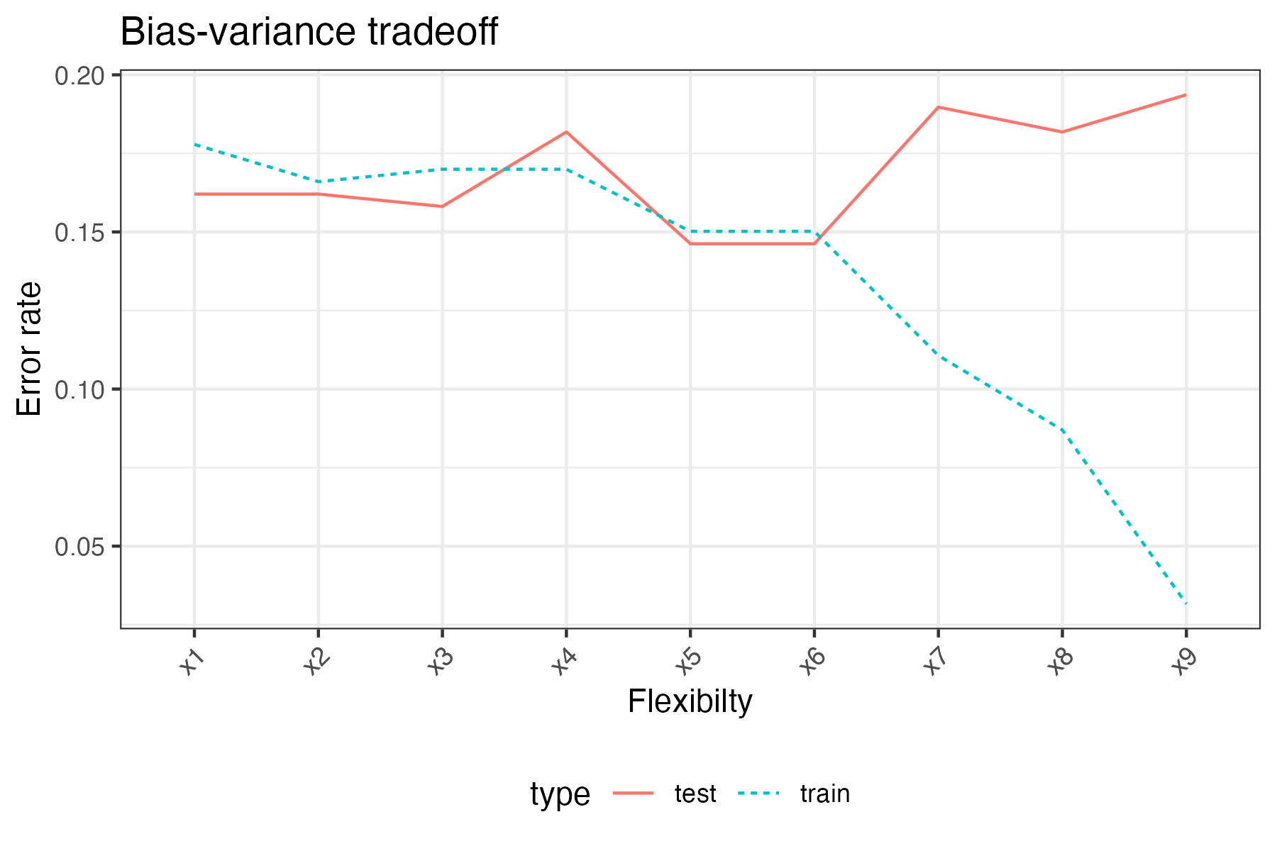
Using this classification script, we create this plot that has the model flexibility on the x-axis and the test error rate on the y-axis.
3.6 Conclusion
Classification asks the same questions as regression, of a different kind of response. Because the response is qualitative, the quantity we estimate is not a number but the probability of each class, \(p_{ic} = P(Y_i = c|X_i)\), collected into \(p_i = f(X_i)\), and a predicted class \(\hat{y}_i\) is read off those estimated probabilities. As in regression, the goal may be prediction, where only the quality of \(\hat{y}_i\) matters, or understanding, where we accept a worse-fitting model in exchange for one whose effect on the class probabilities we can describe.
Evaluation changes with the response. In place of a mean squared error we count the predictions that are wrong, giving a training error rate when those predictions come from the same data used to estimate \(\hat{f}\) and a test error rate when they come from data held out. The training error rate is again the optimistic one, and the test error rate is what we want to be small. Accuracy reports the same information in the opposite direction, and we prefer the error rate so that a larger value always means worse performance.
An error rate counts every mistake the same way, so we also have metrics that separate them. The confusion matrix splits the mistakes by which class was true and which was predicted, and sensitivity, specificity, and precision are ratios read from it: the first two condition on the true class, the third on the predicted class. The log loss instead uses the predicted probabilities themselves, so a confident wrong prediction costs more than a hesitant one.
The bias-variance tradeoff carries over as well. Increasing the flexibility of a classifier drives the training error rate down and eventually drives the test error rate back up, so here too we are choosing a flexibility rather than maximizing one.
Next lecture begins the Regression part of the course with simple linear regression, the first specific choice of \(f\) we make: a straight line in a single explanatory variable, estimated by least squares.