9 Simple Logistic Regression

Learning objectives

After this lecture you should be able to

explain why a linear regression model is a poor model for a binary response,
write the simple logistic regression model in both its probability and log-odds forms, and define the odds of an event,
derive the Bernoulli log-likelihood for $\beta_0$ and $\beta_1$ and explain why, unlike least squares, it has no closed-form maximizer,
fit a simple logistic regression with glm(), predict the probability of the event at a given feature value, and construct a confidence interval for that probability by transforming a log-odds interval through the logistic function,
interpret $\hat\beta_0$ as a log-odds and $\hat\beta_1$ as a change in log-odds, with $e^{\hat\beta_1}$ an odds ratio, and
test $H_0: \beta_1 = 0$ with a $z$-statistic and construct a confidence interval for $\beta_1$ and for the odds ratio $e^{\beta_1}$.

9.1 Binary response

Every model we have fit so far has had a quantitative response. Now take the classification setup from the classification lecture, with $C = 2$ classes, and code the response numerically,

\[Y_i = \begin{cases} 1 & \text{the event of interest occurs for observation } i \\ 0 & \text{otherwise,}\end{cases}\]

where

$Y_i$ is the response for observation $i$, and
“the event of interest” is whichever of the two classes we choose to call a success.

The coding is a choice, and it is not innocent: the model below describes the class coded $1$, so swapping the labels flips the sign of every coefficient.

The expected value of a $0/1$ response is a probability,

\[E[Y_i|X_i] = 1 \cdot P(Y_i = 1|X_i) + 0 \cdot P(Y_i = 0|X_i) = P(Y_i = 1|X_i) \equiv p(X_i),\]

where

$X_i$ is the feature for observation $i$ (a scalar throughout this lecture), and
$p(X_i) = P(Y_i = 1|X_i)$ is the conditional probability that the event occurs.

So modeling the mean of a binary response is modeling a probability, and any model for $p(X)$ has to respect $0 \le p(X) \le 1$ for every $X$.

9.1.1 Credit card default data

Question. Does a customer’s credit card balance tell us whether that customer will default?

Data. ISLR2::Default holds 10,000 credit card customers. The data are simulated rather than observed, and we use them because they are the canonical demonstration of this method. Today we use two of its four variables:

default: did the customer default? A factor with levels No and Yes. This is the response.
balance: the average balance remaining on the card after the monthly payment, in dollars. This is the feature.

Defaulting is the rarer and more consequential outcome, so it is the event of interest: $Y_i = 1$ when customer $i$ defaults. In this sample 3.33% of customers default.

Code

Default <- Default |>
  mutate(default01 = as.numeric(default == "Yes"),
         default_jit = default01 + runif(n(), -0.03, 0.03))

default_plot <- ggplot(Default, aes(x = balance, y = default_jit)) +
  geom_point(alpha = 0.08, size = 0.7) +
  scale_y_continuous(breaks = c(0, 1), labels = c("No (0)", "Yes (1)")) +
  labs(x = "Credit card balance ($)", y = "Default",
       title = "ISLR2::Default")

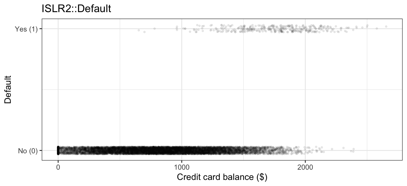
The points are jittered vertically, since every response is exactly $0$ or exactly $1$ and thousands of customers would otherwise stack on top of one another.

No customer with a balance under $652 defaulted, and defaults become steadily more common as the balance grows, while above $2,000 the non-defaulters thin out. Exact proportions cannot be read off jittered points, but the shape can: whatever curve describes $p(\text{balance})$ sits near $0$ on the left, rises through the middle, and has to stay below $1$ on the right.

The obvious next step is to fit the model we already have, by least squares, to this $0/1$ response — expand the note below to see why that does not work.

Linear regression fails

Applying the linear regression model of the earlier lectures to this $0/1$ response gives

\[Y_i = \beta_0 + \beta_1 X_i + \epsilon_i.\]

Since $E[Y_i|X_i] = p(X_i)$, this model says the probability of default is a straight line in balance. Least squares will happily fit that line to the default data, so the fastest way to see what goes wrong is to draw it:

default_lm <- lm(default01 ~ balance, data = Default)

lm_plot <- ggplot(Default, aes(x = balance, y = default_jit)) +
  geom_point(alpha = 0.08, size = 0.7) +
  geom_hline(yintercept = 0, linetype = "dashed", color = "grey40") +
  geom_abline(intercept = coef(default_lm)[1], slope = coef(default_lm)[2],
              color = "#0072B2", linewidth = 1) +
  coord_cartesian(xlim = range(Default$balance),
                  ylim = c(min(fitted(default_lm)) - 0.02, 1.03)) +
  scale_y_continuous(breaks = c(-0.05, 0, 0.5, 1)) +
  labs(x = "Credit card balance ($)", y = "Default (0/1)",
       title = "ISLR2::Default")

zero_crossing <- -coef(default_lm)[1] / coef(default_lm)[2]
percent_negative <- 100 * mean(fitted(default_lm) < 0)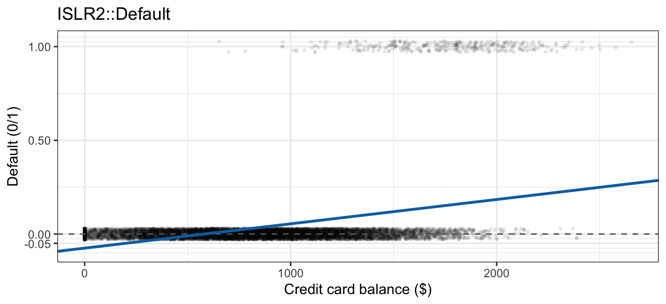

The fitted line drops below the dashed zero line on the left. It crosses zero at a balance of $579, so every customer carrying less than that — 31% of the sample — is assigned a negative estimated probability of default. A negative probability is not a poor estimate; it is not a probability.

Three objections:

Fitted values leave $[0,1]$. A line is unbounded, and $p(X)$ is not. Truncating at $0$ and $1$ after the fact fixes the printed number without fixing the model that produced it.
A constant additive effect cannot be right. The fitted slope says every extra dollar of balance raises the line’s value by the same $0.00013$ regardless of where we start. Wherever the line’s value reaches $0.99$, only $0.01$ of room is left, and just 77 more dollars of balance pushes it past $1$ — a “probability” of more than 100%. A probability has to flatten as it approaches either boundary, and a line never flattens.
The error assumptions fail by construction. $Y_i$ is Bernoulli, not normal, so $\epsilon_i = Y_i - p(X_i)$ takes exactly two values, and \[Var[Y_i|X_i] = p(X_i)\left[1 - p(X_i)\right]\] depends on $X_i$ through $p(X_i)$. Constant variance is impossible unless $p(X)$ is constant. Every standard error, t-test, and interval from lm() rests on assumptions the response itself contradicts.

What we need is a model that is flexible in the middle and bends toward $0$ and $1$ at the ends — the shape the data already showed us.

9.2 Logistic regression model

The simple logistic regression model is

\[p(X) = P(Y = 1|X) = \frac{e^{\beta_0 + \beta_1 X}}{1 + e^{\beta_0 + \beta_1 X}},\]

where

$p(X)$ is the probability the event occurs at feature value $X$,
$\beta_0$ is the intercept on the log-odds scale (defined below), and
$\beta_1$ is the slope on the log-odds scale.

Write $\eta = \beta_0 + \beta_1 X$ for the linear predictor. The function

\[\text{logistic}(\eta) = \frac{e^{\eta}}{1 + e^{\eta}} = \left(1 + e^{-\eta}\right)^{-1}\]

is the logistic function, available in R as plogis() — the second form follows from dividing numerator and denominator of the first by $e^\eta$, and the two are used interchangeably depending on which is easier to work with in a given derivation. The logistic function maps the whole real line into $(0,1)$: $e^{\eta} > 0$ makes $\text{logistic}(\eta) > 0$, and $e^\eta < 1 + e^\eta$ makes $\text{logistic}(\eta) < 1$. As $\eta \to -\infty$, $\text{logistic}(\eta) \to 0$; as $\eta \to \infty$, $\text{logistic}(\eta) \to 1$. The boundary problem raised above is gone no matter what values $\beta_0$, $\beta_1$, and $X$ take.

Beyond this course

The logistic function is not the only function that maps the real line onto $(0,1)$. Replacing it with the standard normal CDF gives probit regression, and the whole family — logistic, probit, Poisson regression, and others — travels under the name generalized linear models; the inverse map, which takes a probability back to the linear predictor, is called the link function. glm() is named for the family, not for logistic regression specifically.

Plotting the curve at a few parameter values shows what $\beta_0$ and $\beta_1$ each control:

Code

shape_data <- tibble(b0 = c(0, 0, 0, -4), b1 = c(1, 2, -1, 1)) |>
  mutate(curve = sprintf("beta[0] == %d * ',' ~ beta[1] == %d", b0, b1)) |>
  mutate(curve = fct_inorder(curve)) |>
  expand_grid(x = seq(-8, 8, length.out = 400)) |>
  mutate(p = plogis(b0 + b1 * x))

logistic_shape_plot <- ggplot(shape_data,
                              aes(x = x, y = p,
                                  color = curve, linetype = curve)) +
  geom_hline(yintercept = c(0, 1), linetype = "dashed", color = "grey60") +
  geom_line(linewidth = 0.9) +
  scale_color_manual(values = c("#E69F00", "#56B4E9", "#009E73", "#CC79A7"),
                     labels = scales::parse_format()) +
  scale_linetype_manual(values = c("solid", "dashed", "dotted", "dotdash"),
                        labels = scales::parse_format()) +
  labs(x = "X", y = "p(X)", color = NULL, linetype = NULL)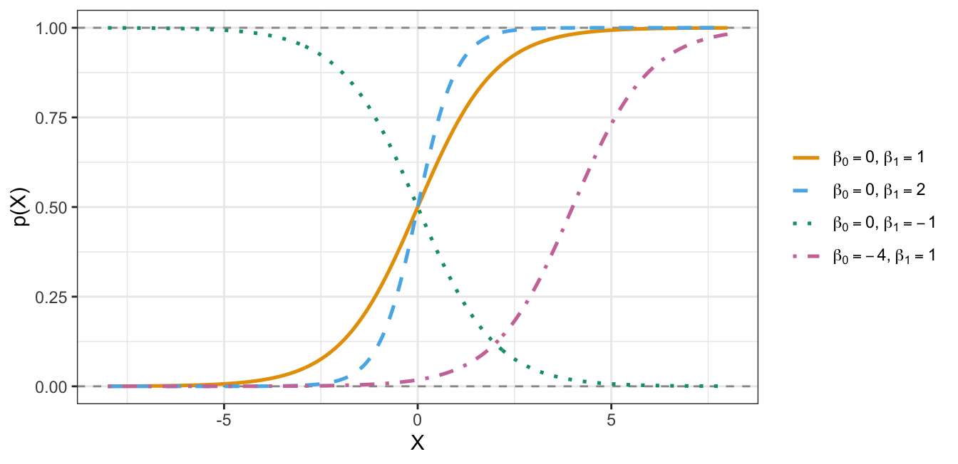

Every curve stays strictly between the two dashed boundaries. Comparing the first two, doubling $\beta_1$ makes the curve rise more steeply without moving where it crosses $0.5$; the third shows that a negative $\beta_1$ reverses the direction; the fourth shows that changing $\beta_0$ shifts the curve horizontally without changing its shape. $\beta_1 = 0$ would give a horizontal line at $\text{logistic}(\beta_0)$: no relationship between $X$ and the probability.

9.2.1 Odds and logit

The odds of an event with probability $p$ are

\[\text{odds} = \frac{p}{1 - p},\]

the ratio of the probability the event happens to the probability it does not. Odds run over $(0, \infty)$: $p = 0.5$ gives odds of $1$, and $p = 0.8$ gives odds of $4$, quoted as “4 to 1.”

Apply this to the logistic model. Since

\[1 - p(X) = 1 - \frac{e^{\beta_0 + \beta_1 X}}{1 + e^{\beta_0 + \beta_1 X}} = \frac{1}{1 + e^{\beta_0 + \beta_1 X}},\]

the odds are

\[\frac{p(X)}{1 - p(X)} = e^{\beta_0 + \beta_1 X}.\]

Taking logarithms,

\[\log\left[\frac{p(X)}{1 - p(X)}\right] = \beta_0 + \beta_1 X.\]

The left side is the logit, or log-odds, of $p(X)$. It is the inverse of the logistic function, and it carries $(0,1)$ onto the whole real line.

This is the payoff of the logistic form. The model is linear — in the parameters and in the feature — once the response is expressed on the log-odds scale, so the entire linear-model vocabulary transfers over. Only the scale on which linearity holds has changed.

9.2.2 Interpreting coefficients

Setting $X = 0$ in the log-odds form gives $\beta_0$ as the log-odds of the event when $X = 0$, so $e^{\beta_0}$ is the odds and $\text{logistic}(\beta_0) = e^{\beta_0}/(1 + e^{\beta_0})$ the probability, at $X = 0$.

Now increase the feature by one unit from an arbitrary $x$:

\[\log\left[\frac{p(x+1)}{1-p(x+1)}\right] - \log\left[\frac{p(x)}{1-p(x)}\right] = \left[\beta_0 + \beta_1 (x+1)\right] - \left[\beta_0 + \beta_1 x\right] = \beta_1.\]

So $\beta_1$ is the change in the log-odds of the event per one-unit increase in $X$. Exponentiating turns the difference into a ratio,

\[\frac{p(x+1)/[1-p(x+1)]}{p(x)/[1-p(x)]} = e^{\beta_1},\]

so $e^{\beta_1}$ is the odds ratio: the multiplicative factor by which the odds of the event change per one-unit increase in $X$. An odds ratio of $1$ ($\beta_1 = 0$) means the odds do not change.

What no coefficient reports is a constant change in the probability, because there isn’t one. Differentiating $p(x) = \text{logistic}(\beta_0 + \beta_1 x)$,

\[\frac{d\, p(x)}{dx} = \beta_1\, p(x)\left[1 - p(x)\right],\]

which depends on $x$ through $p(x)$. It is largest in magnitude, $|\beta_1|/4$, where $p(x) = 0.5$, and it vanishes as $p(x)$ approaches $0$ or $1$ — the flattening a bounded probability needs and a line could never provide. A single number is no more “the effect of $X$ on $p$” here than a single coefficient was the effect of $X$ in a polynomial regression.

9.2.3 Maximum likelihood estimation

Under the model, the observations are independent Bernoulli trials whose success probability depends on the feature,

\[Y_i \stackrel{ind}{\sim} \text{Bernoulli}\left(p(x_i)\right), \qquad i = 1,\ldots,n,\]

so the probability mass function of a single observation is $P(Y_i = y_i|x_i) = p(x_i)^{y_i}\left[1 - p(x_i)\right]^{1-y_i}$ for $y_i \in \{0,1\}$. The likelihood is the product over the sample,

\[L(\beta_0, \beta_1) = \prod_{i=1}^n p(x_i)^{y_i} \left[1 - p(x_i)\right]^{1 - y_i},\]

where

$(x_i, y_i)$ is the observed feature and response for observation $i$, and
$p(x_i) = e^{\beta_0 + \beta_1 x_i}/(1 + e^{\beta_0 + \beta_1 x_i})$ depends on the parameters being estimated.

There is no $\sigma^2$ anywhere: once $p(x_i)$ is specified, the variance $p(x_i)[1-p(x_i)]$ is determined, so the model has exactly two unknown parameters.

Take logarithms, and use the odds identity $p(x_i)/[1 - p(x_i)] = e^{\beta_0 + \beta_1 x_i}$ to simplify:

\[\begin{array}{rl} \ell(\beta_0, \beta_1) &= \displaystyle\sum_{i=1}^n \left\{ y_i \log p(x_i) + (1 - y_i)\log\left[1 - p(x_i)\right] \right\} \\[2mm] &= \displaystyle\sum_{i=1}^n \left\{ y_i \log\left[\frac{p(x_i)}{1 - p(x_i)}\right] + \log\left[1 - p(x_i)\right] \right\} \\[2mm] &= \displaystyle\sum_{i=1}^n \left\{ y_i (\beta_0 + \beta_1 x_i) - \log\left(1 + e^{\beta_0 + \beta_1 x_i}\right) \right\}. \end{array}\]

The maximum likelihood estimators $\hat\beta_0$ and $\hat\beta_1$ are the values maximizing $\ell$. Differentiating,

\[\frac{\partial \ell}{\partial \beta_0} = \sum_{i=1}^n \left[y_i - p(x_i)\right], \qquad \frac{\partial \ell}{\partial \beta_1} = \sum_{i=1}^n x_i\left[y_i - p(x_i)\right],\]

and setting both to zero gives the score equations

\[\sum_{i=1}^n \left[y_i - p(x_i)\right] = 0, \qquad \sum_{i=1}^n x_i\left[y_i - p(x_i)\right] = 0.\]

These say the residuals $y_i - p(x_i)$ sum to zero and are orthogonal to the feature — the same two conditions the least squares normal equations impose. The difference is what happens next. In least squares, $p(x_i)$ would be replaced by $\beta_0 + \beta_1 x_i$, the equations would be linear in $\beta_0$ and $\beta_1$, and solving them would deliver the closed-form least squares estimators of the simple linear regression lecture. Here $p(x_i)$ is a nonlinear function of $\beta_0$ and $\beta_1$, so the equations are nonlinear and no rearrangement produces a closed form.

The estimates are therefore found numerically. The log-likelihood is strictly concave whenever the feature is not constant, so when a maximum exists it is unique, and glm() locates it with an iterative algorithm.

Beyond this course

The algorithm glm() uses is iteratively reweighted least squares (IRLS), which is Newton-Raphson on $\ell$ in disguise: each iteration solves a weighted least squares problem whose weights $p(x_i)[1 - p(x_i)]$ are recomputed from the current estimate. Convergence usually takes a handful of iterations, which is why glm() returns nearly as fast as lm() despite having no formula to evaluate.

Log-likelihood and log loss

Divide the negative log-likelihood by $n$:

\[-\frac{1}{n}\ell(\beta_0,\beta_1) = -\frac{1}{n}\sum_{i=1}^n \left\{ y_i \log p(x_i) + (1 - y_i)\log\left[1 - p(x_i)\right]\right\}.\]

This is exactly the log loss defined in the classification lecture, specialized to $C = 2$ classes and evaluated on the training data. Maximizing the likelihood and minimizing training log loss are the same optimization problem.

9.2.4 Fitting

glm(default ~ balance, data = Default, family = "binomial")

family = "binomial" is what makes this logistic regression; without it, glm() fits a linear model. Two details govern what the coefficients mean:

With a factor response, R models the probability of the second level. Here levels(Default$default) is No, Yes, so glm() models $P(\texttt{default} = \texttt{Yes})$, which is the event we chose.
The response may also be supplied as a $0/1$ numeric vector, with $1$ as the event.

Other ways to write this model

glm() only needs to know which outcome counts as $Y_i = 1$; it does not care how that information is encoded.

default’s second level is already "Yes", since factor levels default to alphabetical order — but relying on alphabetical order to pick the event is fragile. relevel() sets the reference level explicitly, moving the named level to the front so every other level (here, the one level left) is the modeled event regardless of how the factor happened to be built:

Default$default <- relevel(Default$default, ref = "No") # make the reference explicit

The response can also be recoded into a $0/1$ numeric column or a TRUE/FALSE logical column, or compared to the event of interest right inside the formula. All four of the calls below fit identically:

Default$default01 <- as.numeric(Default$default == "Yes") # 0/1 numeric
Default$defaultTF <- Default$default == "Yes"              # TRUE/FALSE logical

glm(default ~ balance, data = Default, family = "binomial")           # factor
glm(default01 ~ balance, data = Default, family = "binomial")         # 0/1 numeric
glm(defaultTF ~ balance, data = Default, family = "binomial")         # logical
glm(default == "Yes" ~ balance, data = Default, family = "binomial")  # comparison

Code

default_prep <- Default |>
  mutate(default = relevel(default, ref = "No"),
         default01 = as.numeric(default == "Yes"),
         defaultTF = default == "Yes")

m_factor     <- glm(default ~ balance, data = default_prep, family = "binomial")
m_numeric    <- glm(default01 ~ balance, data = default_prep, family = "binomial")
m_logical    <- glm(defaultTF ~ balance, data = default_prep, family = "binomial")
m_comparison <- glm(default == "Yes" ~ balance, data = default_prep, family = "binomial")

equivalent_forms_table <- rbind(
  factor     = coef(m_factor),
  "0/1 numeric" = coef(m_numeric),
  "TRUE/FALSE logical" = coef(m_logical),
  comparison = coef(m_comparison)
)

stopifnot(isTRUE(all.equal(coef(m_factor), coef(m_numeric))),
          isTRUE(all.equal(coef(m_factor), coef(m_logical))),
          isTRUE(all.equal(coef(m_factor), coef(m_comparison))))

	(Intercept)	balance
factor	-10.65133	0.005499
0/1 numeric	-10.65133	0.005499
TRUE/FALSE logical	-10.65133	0.005499
comparison	-10.65133	0.005499

The coefficients agree exactly. A logical vector is coerced to $0/1$ with TRUE as $1$, which is exactly what default01 does by hand, and default == "Yes" builds that same logical vector inline without storing it as a column at all. Of the four, the comparison form is often the easiest to read: the formula states the event being modeled directly, rather than leaving it implicit in a factor’s level order or a column name.

Beyond this course

The comparison form generalizes beyond a two-category response. With a response that has more than two categories, glm(y == "target_category" ~ x, family = "binomial") fits a binary logistic regression for that one category against every other category combined, without constructing a separate $0/1$ or logical column first.

Fitting it to the credit card data,

default_glm <- glm(default ~ balance, data = Default, family = "binomial")
coef(default_glm)

  (Intercept)       balance 
-10.651330614   0.005498917

Putting the fitted curve back on the data checks the shape against what the plot suggested. Alongside it, the observed proportion defaulting within $200-wide balance bins gives a model-free estimate of $p(X)$ to compare against; point size shows how many customers are in each bin, since the right-most bins hold very few.

Code

balance_grid <- tibble(balance = seq(0, max(Default$balance), length.out = 400))
balance_grid$p_hat <- predict(default_glm, newdata = balance_grid, type = "response")

binned <- Default |>
  mutate(bin = cut(balance, breaks = seq(0, 2800, by = fit_bin_width),
                   include.lowest = TRUE)) |>
  group_by(bin) |>
  summarize(balance = mean(balance), p = mean(default01), n = n(), .groups = "drop")

fit_plot <- ggplot(Default, aes(x = balance, y = default_jit)) +
  geom_point(alpha = 0.08, size = 0.7) +
  geom_point(data = binned, aes(y = p, size = n), shape = 1, color = "#D55E00") +
  geom_line(data = balance_grid, aes(y = p_hat),
            color = "#0072B2", linewidth = 1) +
  scale_y_continuous(breaks = c(0, 0.5, 1)) +
  scale_size_area(max_size = 5) +
  labs(x = "Credit card balance ($)", y = "P(default = Yes)",
       size = "Customers\nin bin", title = "ISLR2::Default")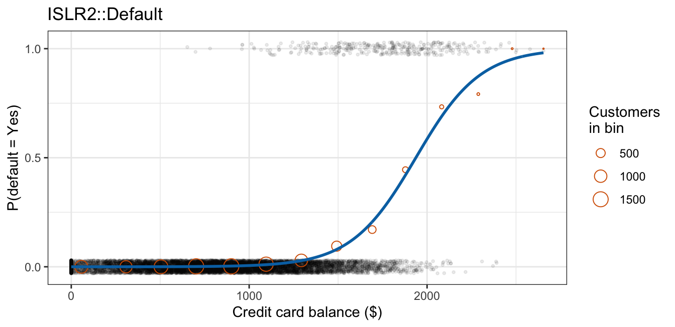

The fitted curve stays inside $[0,1]$ over the full range of balances, sits near zero out to roughly $1,000, and passes through the binned proportions where those bins contain enough customers to be worth reading.

9.2.5 Coefficient inference

The maximum likelihood estimators are approximately normal in large samples, which gives the test statistic

\[z = \frac{\hat\beta_j - \beta_j^0}{\text{SE}(\hat\beta_j)},\]

where

$\beta_j^0$ is the value of $\beta_j$ under the null hypothesis, almost always $0$, and
$\text{SE}(\hat\beta_j)$ is the standard error of $\hat\beta_j$, computed by glm() from the curvature of the log-likelihood at its maximum.

Under $H_0: \beta_j = \beta_j^0$, $z$ is approximately standard normal. The statistic is the same ratio as the t-statistic of the linear regression lectures; the reference distribution is normal rather than $t$ because no separate error variance is estimated and because the normality is asymptotic rather than exact.

glm() reports this test for every coefficient at once:

summary(default_glm)


Call:
glm(formula = default ~ balance, family = "binomial", data = Default)

Coefficients:
              Estimate Std. Error z value Pr(>|z|)    
(Intercept) -1.065e+01  3.612e-01  -29.49   <2e-16 ***
balance      5.499e-03  2.204e-04   24.95   <2e-16 ***
---
Signif. codes:  0 '***' 0.001 '**' 0.01 '*' 0.05 '.' 0.1 ' ' 1

(Dispersion parameter for binomial family taken to be 1)

    Null deviance: 2920.6  on 9999  degrees of freedom
Residual deviance: 1596.5  on 9998  degrees of freedom
AIC: 1600.5

Number of Fisher Scoring iterations: 8

The coefficient table has the same layout as lm()’s, with one visible change: z value and Pr(>|z|) in place of t value and Pr(>|t|), for the reason just given.

Beyond this course

The two deviance lines are the likelihood’s answer to RSS and TSS. For a binary response, the residual deviance is $-2\ell$ evaluated at $\hat\beta_0, \hat\beta_1$, and the null deviance is $-2\ell$ for the intercept-only model. Differences between deviances of nested models play the role that differences in RSS play for an F-test, and AIC penalizes the residual deviance by twice the number of estimated parameters.

An approximate $(1-\alpha)100\%$ confidence interval for $\beta_j$ follows:

\[\hat\beta_j \pm z_{1-\alpha/2}\,\text{SE}(\hat\beta_j),\]

with $z_{1-\alpha/2}$ the $(1-\alpha/2)$ quantile of the standard normal distribution. In R, confint.default() on a fitted glm returns exactly this interval for $\beta_j$. Exponentiating both endpoints gives an interval for the odds ratio $e^{\beta_j}$, because $e^x$ is increasing and therefore preserves the order of the endpoints.

Beyond this course

Plain confint() on a glm object returns a different, profile likelihood interval instead, built from the log-likelihood directly rather than from $\hat\beta_j \pm z_{1-\alpha/2}\text{SE}(\hat\beta_j)$, so it will not match confint.default()’s numbers.

For balance,

z_balance <- summary(default_glm)$coefficients["balance", "z value"]
ci_beta1  <- confint.default(default_glm)["balance", ]

round(z_balance, 2)  # z-statistic for beta_1

[1] 24.95

round(ci_beta1,  5)  # 95% CI for beta_1, per dollar

  2.5 %  97.5 % 
0.00507 0.00593

$z = 24.95$ is far beyond any conventional critical value, so the data are overwhelmingly inconsistent with $\beta_1 = 0$. The confidence interval for $\beta_1$ runs from $0.005067$ to $0.005931$ log-odds per dollar, and exponentiating both endpoints gives an interval for the odds ratio per dollar, entirely above $1$, the odds ratio corresponding to no association.

9.2.6 Prediction

The fitted model returns a probability at any feature value,

\[\hat p(x) = \frac{e^{\hat\beta_0 + \hat\beta_1 x}}{1 + e^{\hat\beta_0 + \hat\beta_1 x}}.\]

In R, predict() on a glm object returns the linear predictor $\hat\beta_0 + \hat\beta_1 x$ by default; type = "response" applies $\text{logistic}(\cdot)$ and returns $\hat p(x)$.

Evaluating $\hat p(x)$ at a few balances spread across the range of the data shows how the three scales — log-odds, odds, and probability — move against one another:

Code

pred_balances <- c(500, 1000, 1500, 2000, 2500)

pred_data <- tibble(balance = pred_balances) |>
  mutate(log_odds = predict(default_glm, newdata = tibble(balance = pred_balances)),
         odds     = exp(log_odds),
         p_hat    = predict(default_glm, newdata = tibble(balance = pred_balances),
                            type = "response"))

pred_table <- pred_data |>
  mutate(log_odds = sprintf("%.2f", log_odds),
         odds     = formatC(odds,  format = "g", digits = 3),
         p_hat    = formatC(p_hat, format = "g", digits = 3)) |>
  knitr::kable(col.names = c("Balance ($)", "Log-odds", "Odds",
                             "Estimated P(default)"),
               align = "cccc")

p_at <- function(x) pred_data$p_hat[pred_data$balance == x]

Balance ($)	Log-odds	Odds	Estimated P(default)
500	-7.90	0.00037	0.00037
1000	-5.15	0.00579	0.00575
1500	-2.40	0.0905	0.0829
2000	0.35	1.41	0.586
2500	3.10	22.1	0.957

The log-odds column increases by the same amount for every $500 step, by construction, and the odds column is multiplied by the same factor. The probability column does neither: the step from $1,500 to $2,000 raises the estimated probability by 0.503, while the identical $500 step from $500 to $1,000 raises it by only 0.005, because down there the curve is still pressed against $0$.

$\hat p(x)$ is itself an estimate, with uncertainty inherited from $\hat\beta_0$ and $\hat\beta_1$. Building a confidence interval for $p(x)$ climbs the same three scales as prediction did above: log-odds, then odds, then probability.

predict() with type = "link" and se.fit = TRUE returns $\hat\eta(x)$ and $\text{SE}(\hat\eta(x))$, giving a Wald interval for the log-odds at $x$, built the same way as the interval for $\beta_1$ above:

\[\hat\eta(x) \pm z_{1-\alpha/2}\,\text{SE}(\hat\eta(x)).\]

Exponentiating both endpoints — the same increasing transform that turned the interval for $\beta_1$ into an interval for the odds ratio $e^{\beta_1}$ — carries this to an interval for the odds at $x$, $\text{odds}(x) = p(x)/[1-p(x)]$. A second increasing transform, $p = \text{odds}/(1+\text{odds})$ — the same map that turns $e^\eta$ into $\text{logistic}(\eta) = e^\eta/(1+e^\eta)$ earlier in this section — carries the odds interval to an interval for $p(x)$ itself.

x0 <- 1500

At a balance of $1,500:

link_x0    <- predict(default_glm, newdata = tibble(balance = x0),
                      type = "link", se.fit = TRUE)
eta_hat_x0 <- link_x0$fit
eta_ci_x0  <- eta_hat_x0 + c(-1, 1) * qnorm(0.975) * link_x0$se.fit
odds_ci_x0 <- exp(eta_ci_x0)
p_ci_x0    <- odds_ci_x0 / (1 + odds_ci_x0)

ci_walkthrough <- tibble(
  Scale    = c("Log-odds", "Odds", "P(default)"),
  Estimate = c(eta_hat_x0, exp(eta_hat_x0), plogis(eta_hat_x0)),
  Lower    = c(eta_ci_x0[1], odds_ci_x0[1], p_ci_x0[1]),
  Upper    = c(eta_ci_x0[2], odds_ci_x0[2], p_ci_x0[2])
) |>
  mutate(across(c(Estimate, Lower, Upper), \(x) sprintf("%.4f", x))) |>
  knitr::kable(col.names = c("Scale", "Estimate", "2.5%", "97.5%"),
               align = "lccc")

Scale	Estimate	2.5%	97.5%
Log-odds	-2.4030	-2.5441	-2.2618
Odds	0.0905	0.0785	0.1042
P(default)	0.0829	0.0728	0.0943

The composition of two increasing transforms is increasing, so this two-step route lands on the same interval as applying $\text{logistic}(\cdot)$ directly to the $\eta(x)$ endpoints in one step — the shortcut used to build the whole band below. This is a pointwise interval: each vertical slice is a separate 95% interval for $p(x)$ at that one balance, not a region covering the whole curve at once.

Code

band_grid <- tibble(balance = seq(0, max(Default$balance), length.out = 400))

band_link <- predict(default_glm, newdata = band_grid,
                     type = "link", se.fit = TRUE)

band_grid <- band_grid |>
  mutate(eta   = band_link$fit,
         se    = band_link$se.fit,
         p_hat = plogis(eta),
         lower = plogis(eta - qnorm(0.975) * se),
         upper = plogis(eta + qnorm(0.975) * se))

confidence_band_plot <- ggplot(band_grid, aes(x = balance, y = p_hat)) +
  geom_ribbon(aes(ymin = lower, ymax = upper), fill = "grey70", alpha = 0.6) +
  geom_line(color = "#0072B2", linewidth = 1) +
  scale_y_continuous(breaks = c(0, 0.5, 1)) +
  labs(x = "Credit card balance ($)", y = "P(default = Yes)",
       title = "ISLR2::Default")

peak_balance <- band_grid$balance[which.max(band_grid$upper - band_grid$lower)]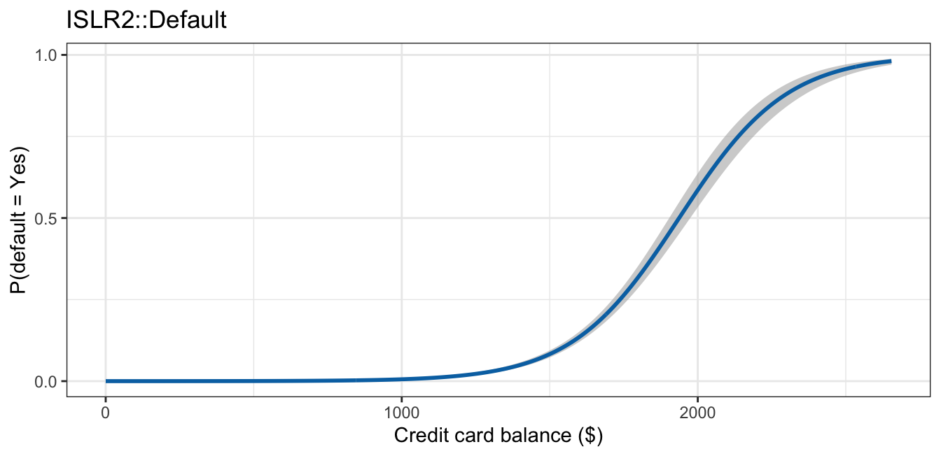

The gray band is squeezed to a hairline at both ends, where the curve is pinned near $0$ or near $1$ regardless of the exact coefficients, and is widest through the steep middle, peaking near a balance of $2,042. This is not because the coefficients are estimated less precisely there — the standard error of $\hat\eta(x)$ is actually smallest near the middle of the balance range and largest at the two ends — but because a fixed-width interval on the log-odds scale converts to a wider probability-scale interval exactly where the logistic curve is steepest, and to a narrower one where it is nearly flat against $0$ or $1$. This is also why the band is not symmetric around the curve the way a linear regression’s confidence interval for the mean response would be.

9.3 Credit card default probability

Question. Does a customer’s credit card balance predict whether they default, and by how much?

Data. ISLR2::Default again: 10,000 credit card customers, default as the response (3.33% default), and balance as the feature.

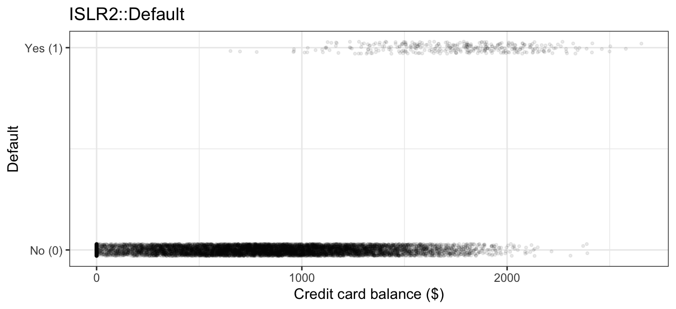
Defaults are rare at low balances and steadily more common as balance climbs, the shape a probability model needs to reproduce.

9.3.1 Fitting

Fitting $\texttt{default} \sim \texttt{balance}$ by logistic regression,

coef(default_glm)

  (Intercept)       balance 
-10.651330614   0.005498917

summary(default_glm)


Call:
glm(formula = default ~ balance, family = "binomial", data = Default)

Coefficients:
              Estimate Std. Error z value Pr(>|z|)    
(Intercept) -1.065e+01  3.612e-01  -29.49   <2e-16 ***
balance      5.499e-03  2.204e-04   24.95   <2e-16 ***
---
Signif. codes:  0 '***' 0.001 '**' 0.01 '*' 0.05 '.' 0.1 ' ' 1

(Dispersion parameter for binomial family taken to be 1)

    Null deviance: 2920.6  on 9999  degrees of freedom
Residual deviance: 1596.5  on 9998  degrees of freedom
AIC: 1600.5

Number of Fisher Scoring iterations: 8

Both coefficients are far from zero relative to their standard errors, exactly as the $z$-test above found.

9.3.2 Estimated odds ratios

Code

b         <- coef(default_glm)
or_dollar <- unname(exp(b["balance"]))
or_100    <- unname(exp(100 * b["balance"]))
ci_or_100 <- exp(100 * ci_beta1)

The estimated log-odds of default are

\[\log\left[\frac{\hat p(X)}{1 - \hat p(X)}\right] = -10.65 + 0.005499 \times \texttt{balance}.\]

The intercept $\hat\beta_0 = -10.65$ is the estimated log-odds of default for a customer carrying no balance, which corresponds to estimated odds of $e^{-10.65} = 0.0000237$ and an estimated probability of $0.0000237$ — odds and probability agree to three significant digits here because $p/(1-p) \approx p$ whenever $p$ is small. Unlike many intercepts, this one describes customers who actually exist: 499 customers in this sample carry a zero balance, and 0 of them defaulted.

The slope $\hat\beta_1 = 0.005499$ is positive, so every additional dollar of balance raises the log-odds of default by $0.005499$ — equivalently, multiplies the odds of default by $e^{\hat\beta_1} = 1.00551$.

A dollar is too small a unit to read comfortably, and nothing forces us to use it: balance can be rescaled by any positive constant without changing the model, since $\beta_1 X = (100\beta_1)(X/100)$ — measuring balance in hundreds of dollars instead of dollars multiplies the slope by $100$ and leaves the fitted probabilities untouched. Scaling up this way, an additional $100 of balance multiplies the odds of default by

\[e^{100\hat\beta_1} = 1.73,\]

a 73% increase in the odds of default per $100. It is not a 73% increase in the probability of default; the change in probability depends on the balance you started from. $100 is simply the increment a person managing a credit line can picture without doing arithmetic first.

The same rescaling applies to the confidence interval: from the coefficient inference above, multiplying the endpoints of the interval for $\beta_1$ by $100$ and exponentiating gives $(1.66, 1.81)$ on the per-$100 odds-ratio scale, every value of it well above $1$.

9.3.3 Fitted probability

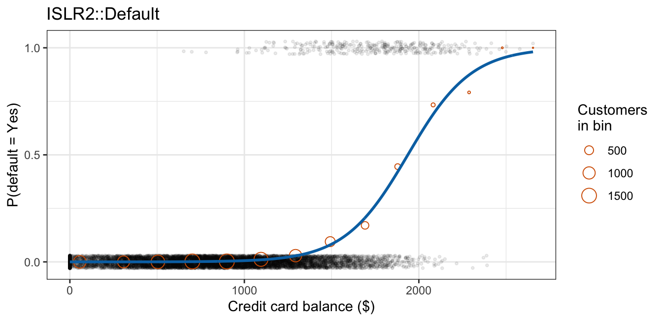
The fitted curve stays inside $[0,1]$ everywhere, and tracks the binned observed proportions closely wherever a bin holds enough customers to estimate one.

9.4 Conclusion

Simple logistic regression models a binary response’s probability as the logistic function of a linear predictor, $p(X) = \text{logistic}(\beta_0 + \beta_1 X)$, equivalently a statement that the log-odds of the event are linear in $X$. Estimation is by maximum likelihood rather than least squares because a Bernoulli response has a variance determined by its own mean, which breaks the least squares error assumptions by construction; and because $p(x_i)$ is a nonlinear function of $\beta_0$ and $\beta_1$, the score equations have no closed-form solution, so glm() finds $\hat\beta_0$ and $\hat\beta_1$ numerically.

Coefficients are read on the log-odds scale — $\beta_0$ as a baseline log-odds, $\beta_1$ as a change in log-odds per unit of $X$ — and exponentiated into odds ratios for a multiplicative statement about the odds. Neither describes a constant change in probability, because the logistic curve has no constant slope. The same increasing-transform idea that turns a log-odds interval into an odds-ratio interval also turns a confidence interval for the linear predictor at a point into a confidence interval for the predicted probability there, one increasing map — exponentiate, then odds-to-probability — at a time.

The next lecture keeps this model and adds features: multiple logistic regression asks what each feature contributes once the others are held fixed, the same question multiple linear regression asked of a quantitative response.