10 Multiple Logistic Regression

Learning objectives

After this lecture you should be able to

write the multiple logistic regression model in its probability and log-odds forms using the linear predictor $x_i\beta$, and encode a two-level categorical feature as an indicator against a reference level,
interpret $\beta_j$ as a change in log-odds and $e^{\beta_j}$ as an odds ratio holding every other feature fixed, and distinguish that from the interpretation of the same feature’s coefficient fit alone,
fit an additive multiple logistic regression with glm(), predict $\hat p(x)$ for a specified combination of feature values, and construct a confidence interval for that probability by transforming a log-odds interval to the odds scale and then to the probability scale,
test $H_0: \beta_j = 0$ with a $z$-statistic and interpret a confidence interval for the odds ratio $e^{\beta_j}$ as a statement about feature $j$ after accounting for the other features,
conduct a drop-in-deviance test comparing two nested logistic regression models and explain its parallel with the F-test comparing two nested linear regression models, and
diagnose a coefficient whose sign reverses between a one-feature and a multi-feature model as confounding, and explain the mechanism from descriptive summaries of the features.

10.1 Multiple features

The previous lecture modeled the probability of default from a single feature, credit card balance. ISLR2::Default records two more variables on the same 10,000 customers:

student: is the customer a student? A factor with levels No and Yes.
income: the customer’s income, in dollars. This one is set aside for this lecture; everything below uses balance and student.

Having more than one feature raises a question that a one-feature model cannot answer: what does each feature tell us that the others do not? This lecture answers it for an additive model, in which each feature contributes its own term to the linear predictor.

10.1.1 Categorical features

A categorical feature enters a logistic regression exactly as it enters a multiple linear regression: through dummy variables against a reference level. A feature with $L$ levels contributes $L-1$ indicators, and the level left without an indicator is the reference.

student has two levels, so it contributes one indicator. Taking No as the reference level,

\[D_i = \mathrm{I}(\texttt{student}_i = \texttt{Yes}) = \begin{cases} 1 & \text{customer } i \text{ is a student} \\ 0 & \text{otherwise,}\end{cases}\]

where

$D_i$ is the indicator for observation $i$, and
$\mathrm{I}(\cdot)$ is $1$ when its argument is true and $0$ otherwise.

R builds this column automatically from a factor, using the first level as the reference, and names the coefficient after the level being indicated — studentYes below.

10.1.2 Student status and default

Question. Are students more likely to default than non-students?

Data. The same 10,000 customers as in the previous lecture, now using student as the feature and default as the response, with $Y_i = 1$ when customer $i$ defaults.

Code

Default <- Default |>
  mutate(default01 = as.numeric(default == "Yes"),
         default_jit = default01 + runif(n(), -0.03, 0.03))

student_rates <- Default |>
  group_by(student) |>
  summarize(n = n(),
            defaults = sum(default01),
            rate = mean(default01),
            .groups = "drop")

student_rate_table <- student_rates |>
  mutate(n = format(n, big.mark = ","),
         rate = sprintf("%.2f%%", 100 * rate)) |>
  knitr::kable(col.names = c("Student", "Customers", "Defaults",
                             "Percent defaulting"),
               align = "cccc")

rate_of <- function(s) student_rates$rate[student_rates$student == s]

Student	Customers	Defaults	Percent defaulting
No	7,056	206	2.92%
Yes	2,944	127	4.31%

Students default at 4.31% versus 2.92% for non-students, so the student default rate is 1.48 times the non-student rate. That is a ratio of rates, not of odds; the two happen to be close here only because both rates are small.

Fitting the simple logistic regression with $D$ as the feature turns that comparison into a coefficient:

student_glm <- glm(default ~ student, data = Default, family = "binomial")
coef(student_glm)

(Intercept)  studentYes 
 -3.5041278   0.4048871

Code

bs <- coef(student_glm)
or_student_alone <- unname(exp(bs["studentYes"]))
ci_student_alone <- exp(confint.default(student_glm)["studentYes", ])

The estimated log-odds of default are

\[\log\left[\frac{\hat p(D)}{1 - \hat p(D)}\right] = -3.50 +0.405 \, D.\]

With a single indicator feature, the two fitted values are the two observed log-odds. The intercept $\hat\beta_0 = -3.50$ is the log-odds of default among non-students, and $\hat\beta_0 + \hat\beta_1$ is the log-odds among students. The coefficient $\hat\beta_1 = 0.405$ is the difference between them, so $e^{\hat\beta_1} = 1.50$ is the odds of default for a student divided by the odds for a non-student. The confidence interval for that odds ratio runs from 1.20 to 1.88, entirely above $1$.

Conclusion. Taken by itself, student status is associated with a 50% increase in the odds of default.

10.1.3 Balance and student together

The previous lecture found balance strongly associated with default; this lecture has now found student status associated with default as well. Before putting both in one model, start with the individual customers rather than a summary of them: the same jittered scatter of default against balance from the previous lecture, now split into two panels by student status.

Code

raw_plot <- ggplot(Default, aes(x = balance, y = default_jit)) +
  geom_point(alpha = 0.08, size = 0.7) +
  facet_wrap(~ student, labeller = label_both) +
  scale_y_continuous(breaks = c(0, 1), labels = c("No (0)", "Yes (1)")) +
  labs(x = "Credit card balance ($)", y = "Default",
       title = "ISLR2::Default")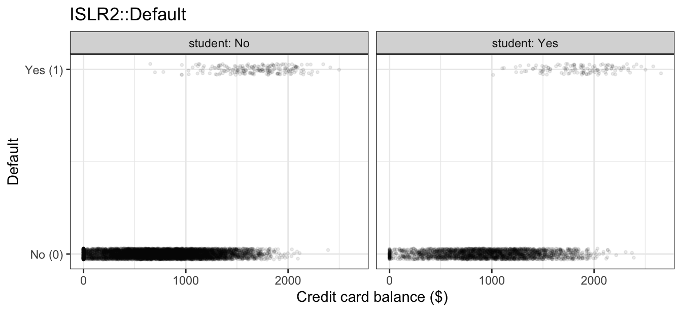

The student panel’s points sit further right on average, a first hint of a balance difference between the two groups, but with 2,944 students against 7,056 non-students plotted at the same jitter and transparency, that shift is hard to read precisely by eye. Two descriptive summaries make it precise.

The first compares the distribution of balance for students and non-students.

Code

balance_means <- Default |>
  group_by(student) |>
  summarize(mean_balance = mean(balance), .groups = "drop")

balance_density_plot <- ggplot(Default,
                               aes(x = balance,
                                   color = student, linetype = student)) +
  geom_density(linewidth = 0.9) +
  geom_vline(data = balance_means,
             aes(xintercept = mean_balance,
                 color = student, linetype = student),
             linewidth = 0.5, show.legend = FALSE) +
  scale_color_manual(values = c("#0072B2", "#D55E00")) +
  labs(x = "Credit card balance ($)", y = "Density",
       color = "Student", linetype = "Student",
       title = "ISLR2::Default")

mean_balance_of <- function(s) {
  balance_means$mean_balance[balance_means$student == s]
}

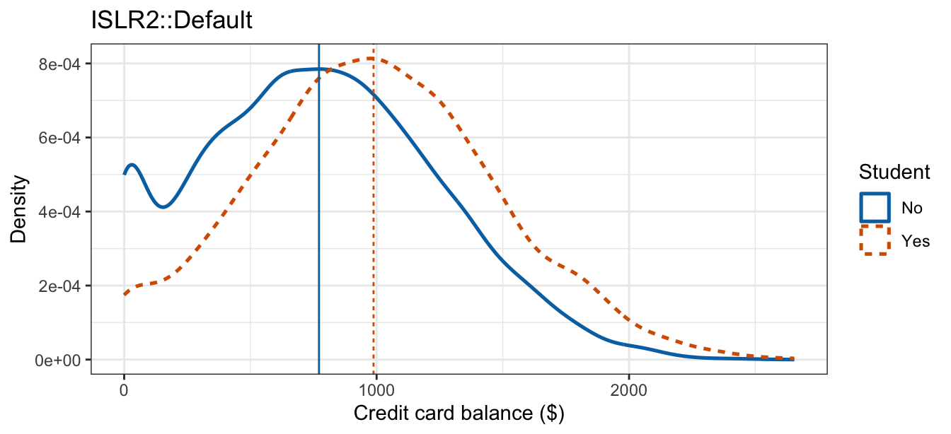
The two densities are shifted relative to one another, with the vertical lines marking the group means: students average $988 versus $772 for non-students, a difference of $216. Students carry more balance.

The second summary asks what happens to the default rate within a narrow range of balance. Splitting balance into $400-wide bins and computing the observed default rate separately for students and non-students within each bin gives a model-free comparison of two customers who carry similar balances. Bins holding too few customers of a given student status to estimate a rate are dropped.

Code

binned_rates <- Default |>
  mutate(bin = cut(balance, breaks = seq(0, 2800, by = bin_width),
                   include.lowest = TRUE)) |>
  group_by(student, bin) |>
  summarize(balance = mean(balance), rate = mean(default01), n = n(),
            .groups = "drop") |>
  filter(n >= min_bin_n)

binned_plot <- ggplot(binned_rates,
                      aes(x = balance, y = rate,
                          color = student, shape = student,
                          linetype = student)) +
  geom_line(linewidth = 0.9) +
  geom_point(size = 2.5) +
  scale_color_manual(values = c("#0072B2", "#D55E00")) +
  labs(x = "Mean balance within bin ($)",
       y = "Observed proportion defaulting",
       color = "Student", shape = "Student", linetype = "Student",
       title = paste0("ISLR2::Default, $", bin_width, "-wide balance bins"))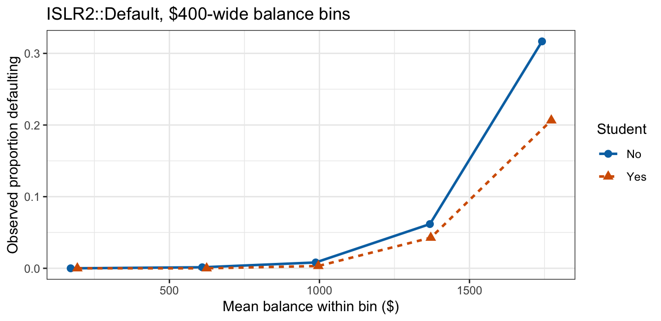

Within every bin shown, the student curve sits at or below the non-student curve. Comparing customers who carry similar balances reverses the direction of the association that the aggregate rates showed. The curves stop near $1,773 because every bin beyond that holds fewer than 100 customers in at least one of the two groups.

Neither summary used a model. Together they say that students carry higher balances, that higher balances default more, and that at a fixed balance students default less; a model with both features lets us separate those statements.

10.2 Multiple logistic regression model

Let $x_{i1}, \ldots, x_{ip}$ be the $p$ features recorded on observation $i$. The multiple logistic regression model is

\[p(x_i) = P(Y_i = 1|x_i) = \frac{e^{\beta_0 + \beta_1 x_{i1} + \cdots + \beta_p x_{ip}}}{1 + e^{\beta_0 + \beta_1 x_{i1} + \cdots + \beta_p x_{ip}}},\]

where

$p(x_i)$ is the probability the event occurs for observation $i$,
$x_{ij}$ is the value of feature $j$ for observation $i$, and
$\beta_0, \beta_1, \ldots, \beta_p$ are the regression coefficients.

The same algebra as in the previous lecture — form $1 - p(x_i)$, divide, take logarithms — puts the model in its log-odds form,

\[\log\left[\frac{p(X)}{1 - p(X)}\right] = \beta_0 + \beta_1 X_1 + \cdots + \beta_p X_p.\]

The right side is exactly the linear predictor of the multiple linear regression lecture. Using that lecture’s model matrix notation together with the linear predictor $\eta$ of the previous lecture,

$x_i = (1, x_{i1}, \ldots, x_{ip})$ is the $i$th row of the $n \times (p+1)$ model matrix $\mathbf{X}$,
$\beta = (\beta_0, \ldots, \beta_p)^\top$ is the vector of coefficients, and
$\eta = \mathbf{X}\beta$ is the $n$-vector of linear predictors, with $i$th element $\eta_i = x_i\beta$,

the model is

\[p(x_i) = \text{logistic}(x_i\beta) = \frac{e^{x_i\beta}}{1 + e^{x_i\beta}}.\]

So multiple logistic regression is multiple linear regression’s linear predictor passed through the logistic function. Everything the linear predictor can express — several quantitative features, dummy variables for categorical features, polynomial terms, step functions — is available here unchanged, because none of it touches the logistic function wrapped around it.

The model above is additive: each feature contributes its own term $\beta_j x_{ij}$ to $\eta_i$, and no term involves two features at once.

10.2.1 Maximum likelihood estimation

The observations are still independent Bernoulli trials, $Y_i \stackrel{ind}{\sim} \text{Bernoulli}(p(x_i))$, so the log-likelihood derived in the previous lecture carries over with $\beta_0 + \beta_1 x_i$ replaced by $x_i\beta$:

\[\ell(\beta) = \ell(\beta_0, \beta_1, \ldots, \beta_p) = \sum_{i=1}^n \left\{ y_i \, x_i\beta - \log\left(1 + e^{x_i\beta}\right)\right\},\]

where

$x_i = (1, x_{i1}, \ldots, x_{ip})$ is the observed feature row for observation $i$, and
$y_i \in \{0, 1\}$ is the observed response.

Nothing structural changed. There are now $p+1$ parameters rather than $2$, still no $\sigma^2$, and still no closed-form maximizer, because $p(x_i)$ remains a nonlinear function of the coefficients. The maximum likelihood estimator $\hat\beta$ is the maximizer of $\ell$, and glm() finds it numerically by the same iterative algorithm as before.

Differentiating with respect to $\beta_j$ and setting the result to zero gives one score equation per coefficient,

\[\sum_{i=1}^n x_{ij}\left[y_i - p(x_i)\right] = 0, \qquad j = 0, 1, \ldots, p,\]

with $x_{i0} = 1$. As in the one-feature case, these say the residuals $y_i - p(x_i)$ sum to zero and are orthogonal to every feature — the same conditions the least squares normal equations impose, though here the equations are nonlinear in $\beta$.

10.2.2 Interpreting coefficients

Fix the values of all features other than $X_j$ and increase $X_j$ by one unit. On the log-odds scale, every term except the $j$th is identical on both sides, so the difference is

\[\left[\beta_0 + \cdots + \beta_j(x_j + 1) + \cdots + \beta_p x_p\right] - \left[\beta_0 + \cdots + \beta_j x_j + \cdots + \beta_p x_p\right] = \beta_j.\]

So $\beta_j$ is the change in the log-odds of the event per one-unit increase in $X_j$ holding every other feature fixed, and exponentiating, $e^{\beta_j}$ is the multiplicative change in the odds of the event per one-unit increase in $X_j$ holding every other feature fixed.

The qualifier is the whole difference between this lecture and the last one, and it is the same qualifier that attaches to a multiple linear regression coefficient. The cancellation above is what licenses it: the comparison $\beta_j$ describes is between two observations that differ in $X_j$ and agree on everything else in the model.

Two consequences follow.

$\beta_j$ from a multi-feature fit and from a one-feature fit answer different questions. Fit alone, a feature’s coefficient describes the comparison between observations that differ in that feature and in whatever else happens to vary with it. In an additive model, it describes the comparison holding the other included features fixed. The two can differ in magnitude, and they can differ in sign.
“Holding fixed” covers only features in the model. A variable not in $X$ is not held fixed by including other features, so a coefficient never describes a comparison that adjusts for something the model never saw.

For a dummy variable — a feature $X_j$ taking only the values $0$ and $1$ — a “one-unit increase” is the change from the reference level to the indicated level, so $e^{\beta_j}$ is the odds of the event at that level divided by the odds at the reference level, again holding the other features fixed.

The intercept $\beta_0$ is the log-odds of the event when every feature is $0$ — for a dummy variable, when the observation is at the reference level.

10.2.3 Fitting

glm(default ~ balance + student, data = Default, family = "binomial")

The + makes the model additive: balance and student each contribute one term to the linear predictor. Terms joined by * or : would add products of features, which the additive model excludes.

Fitting it to the credit card data,

additive_glm <- glm(default ~ balance + student, data = Default,
                    family = "binomial")
coef(additive_glm)

  (Intercept)       balance    studentYes 
-10.749495878   0.005738104  -0.714877620

3 coefficients are estimated for $p = 2$ features, and the third is named studentYes: R built the indicator $D$ from the factor and took No as the reference level, as promised above. Writing $X_1 = \texttt{balance}$ and $X_2 = D$, the three estimates are $\hat\beta_0$, $\hat\beta_1$, and $\hat\beta_2$.

10.2.4 Coefficient inference

Inference proceeds coefficient by coefficient with the same machinery as the previous lecture. Maximum likelihood estimators are approximately normal in large samples, so

\[z = \frac{\hat\beta_j - \beta_j^0}{\text{SE}(\hat\beta_j)}\]

is approximately standard normal under $H_0: \beta_j = \beta_j^0$, where

$\beta_j^0$ is the null value, almost always $0$, and
$\text{SE}(\hat\beta_j)$ is the standard error computed by glm() from the curvature of the log-likelihood at $\hat\beta$.

An approximate $(1-\alpha)100\%$ confidence interval is $\hat\beta_j \pm z_{1-\alpha/2}\text{SE}(\hat\beta_j)$, and exponentiating both endpoints gives an interval for the odds ratio $e^{\beta_j}$.

Every one of these statements is about $\beta_j$ with the other features in the model held fixed, so the test of $H_0: \beta_j = 0$ asks whether feature $j$ is associated with the response after accounting for the other features — not whether it is associated with the response at all.

glm() reports the test for every coefficient at once:

summary(additive_glm)


Call:
glm(formula = default ~ balance + student, family = "binomial", 
    data = Default)

Coefficients:
              Estimate Std. Error z value Pr(>|z|)    
(Intercept) -1.075e+01  3.692e-01 -29.116  < 2e-16 ***
balance      5.738e-03  2.318e-04  24.750  < 2e-16 ***
studentYes  -7.149e-01  1.475e-01  -4.846 1.26e-06 ***
---
Signif. codes:  0 '***' 0.001 '**' 0.01 '*' 0.05 '.' 0.1 ' ' 1

(Dispersion parameter for binomial family taken to be 1)

    Null deviance: 2920.6  on 9999  degrees of freedom
Residual deviance: 1571.7  on 9997  degrees of freedom
AIC: 1577.7

Number of Fisher Scoring iterations: 8

Code

ba <- coef(additive_glm)
or_balance_100 <- unname(exp(100 * ba["balance"]))
or_student_adj <- unname(exp(ba["studentYes"]))
ci_adj <- confint.default(additive_glm)
ci_or_student_adj <- exp(ci_adj["studentYes", ])
ci_or_balance_100 <- exp(100 * ci_adj["balance", ])
z_student_adj <- summary(additive_glm)$coefficients["studentYes", "z value"]
p_student_adj <- summary(additive_glm)$coefficients["studentYes", "Pr(>|z|)"]

Collecting the two tests and the two odds ratios on interpretable scales:

Code

inference_table <- tibble(
  coefficient = c("balance (per $100)", "student (Yes vs. No)"),
  estimate    = c(100 * ba["balance"], ba["studentYes"]),
  z           = summary(additive_glm)$coefficients[c("balance", "studentYes"),
                                                   "z value"],
  odds_ratio  = c(or_balance_100, or_student_adj),
  lower       = c(ci_or_balance_100[1], ci_or_student_adj[1]),
  upper       = c(ci_or_balance_100[2], ci_or_student_adj[2])
) |>
  mutate(across(c(estimate, z, odds_ratio, lower, upper),
                \(x) sprintf("%.3f", x))) |>
  knitr::kable(col.names = c("Coefficient", "Estimate (log-odds)", "z",
                             "Odds ratio", "95% CI lower", "95% CI upper"),
               align = "lccccc")

Coefficient	Estimate (log-odds)	z	Odds ratio	95% CI lower	95% CI upper
balance (per $100)	0.574	24.750	1.775	1.696	1.858
student (Yes vs. No)	-0.715	-4.846	0.489	0.366	0.653

Both $z$-statistics are far from zero. The interval for the balance odds ratio per $100 lies entirely above $1$, and the interval for the student odds ratio lies entirely below $1$, running from 0.37 to 0.65.

10.2.5 Drop-in-deviance test

A $z$-statistic tests one coefficient at a time. Asking whether a group of coefficients is all zero at once — every dummy variable of a five-level categorical feature, say — requires comparing two models rather than reading one row of a coefficient table.

The multiple linear regression lecture answered that question with an F-test: fit a reduced model without the group and a full model with it, and compare their residual sums of squares. Logistic regression has no residual sum of squares, but it has the quantity that plays the same role.

For a binary response, the residual deviance of a fitted logistic regression is

\[D = -2\,\ell(\hat\beta),\]

where

$\ell$ is the Bernoulli log-likelihood above and
$\hat\beta$ is the maximum likelihood estimate.

glm() prints it as Residual deviance in the summary above, alongside Null deviance, which is $-2\ell$ for the intercept-only model. Smaller deviance means a larger maximized likelihood. Because a reduced model’s coefficients are a special case of the full model’s (the dropped ones fixed at zero), the full model’s maximized likelihood is at least as large, so adding features cannot increase the deviance — exactly as adding features cannot increase RSS in a linear model.

The drop-in-deviance statistic compares a reduced model, nested in a full model with $k$ more parameters, by

\[G^2 = D_r - D_f,\]

where

$D_r$ is the residual deviance of the reduced model, and
$D_f$ is the residual deviance of the full model.

Under $H_0$ that the reduced model is adequate — that all $k$ of the dropped coefficients are zero — $G^2$ is approximately $\chi^2$ with $k$ degrees of freedom in large samples, and the $p$-value is the upper tail probability $P(\chi^2_k > G^2)$.

Two differences from the F-test are worth naming. The F-statistic divides the drop in RSS per degree of freedom by $\hat\sigma^2_f$, because a linear model has an error variance to estimate; a logistic regression has none, so $G^2$ needs no such divisor and carries $k$ in its reference distribution instead. And the F-distribution is exact under normal errors, while the $\chi^2$ reference distribution here is a large-sample approximation.

In R, anova() on two fitted models with test = "Chisq" performs the test. Applying it to this lecture’s two models — reduced default ~ balance, full default ~ balance + student — tests $H_0: \beta_2 = 0$, that student status adds nothing once balance is in the model:

balance_glm <- glm(default ~ balance, data = Default, family = "binomial")
anova(balance_glm, additive_glm, test = "Chisq")

Analysis of Deviance Table

Model 1: default ~ balance
Model 2: default ~ balance + student
  Resid. Df Resid. Dev Df Deviance  Pr(>Chi)    
1      9998     1596.5                          
2      9997     1571.7  1    24.77 6.459e-07 ***
---
Signif. codes:  0 '***' 0.001 '**' 0.01 '*' 0.05 '.' 0.1 ' ' 1

The same numbers assembled from the deviances directly:

G2    <- deviance(balance_glm) - deviance(additive_glm)
k     <- length(coef(additive_glm)) - length(coef(balance_glm))
p_dev <- pchisq(G2, df = k, lower.tail = FALSE)

data.frame(G2 = G2, k = k, p_value = p_dev)

        G2 k      p_value
1 24.77009 1 6.459215e-07

Adding student to the balance-only model drops the deviance by $G^2 = 24.77$ on $k = 1$ degree of freedom, giving $p = 6.5 \times 10^{-7}$. The data are strongly inconsistent with a model in which student status contributes nothing beyond balance.

The $z$-test from the coefficient table tests the same $H_0$, since the two models differ by one coefficient. It gives $z = -4.85$, so $z^2 = 23.48$ against $G^2 = 24.77$, and $p = 1.3 \times 10^{-6}$ against $p = 6.5 \times 10^{-7}$. The two agree on the conclusion without agreeing to the digit, and there is no reason they should: they are different statistics, each approximately $\chi^2_1$ under the null rather than exactly equal to one another.

When the two models differ by more than one coefficient, no single $z$-test answers the question and the drop-in-deviance test is the tool that does. Comparing the intercept-only model to the additive model, for instance, tests $H_0: \beta_1 = \beta_2 = 0$ with $k = 2$, and the two deviances needed are the Null deviance and Residual deviance lines already printed in the summary above.

Beyond this course

$G^2$ is a likelihood-ratio statistic: because $D_r - D_f = -2\left[\ell(\hat\beta_r) - \ell(\hat\beta_f)\right] = -2\log\left(L(\hat\beta_r)/L(\hat\beta_f)\right)$, the test compares the maximized likelihoods of the two models. Wilks’ theorem supplies the $\chi^2_k$ limiting distribution. The per-coefficient $z$-test is a Wald test instead, built from $\hat\beta_j$ and its standard error rather than from the likelihood at two parameter values, which is why the two statistics differ in finite samples while sharing a null distribution in the limit.

10.2.6 Prediction

The fitted model returns a probability for any combination of feature values,

\[\hat p(x) = \frac{e^{x\hat\beta}}{1 + e^{x\hat\beta}},\]

where $x = (1, x_1, \ldots, x_p)$ is a row of feature values. In R, predict() with type = "response" applies the logistic function; the newdata argument takes a data frame with one column per feature, and a categorical feature must be supplied at one of its observed levels.

Evaluating $\hat p(x)$ for a student and a non-student at three balances gives six predictions, and the odds ratio between the two customers at each balance:

Code

pred_grid <- expand_grid(balance = c(1000, 1500, 2000),
                         student = factor(c("No", "Yes"),
                                          levels = levels(Default$student)))
pred_grid$p_hat <- predict(additive_glm, newdata = pred_grid,
                           type = "response")

pred_table <- pred_grid |>
  pivot_wider(names_from = student, values_from = p_hat,
              names_prefix = "student_") |>
  mutate(odds_ratio = (student_Yes / (1 - student_Yes)) /
                      (student_No  / (1 - student_No))) |>
  mutate(across(c(student_No, student_Yes), \(x) sprintf("%.4f", x)),
         odds_ratio = sprintf("%.3f", odds_ratio),
         balance = format(balance, big.mark = ",")) |>
  knitr::kable(col.names = c("Balance ($)", "Non-student", "Student",
                             "Odds ratio"),
               align = "cccc")

p_at <- function(b, s) {
  pred_grid$p_hat[pred_grid$balance == b & pred_grid$student == s]
}

Balance ($)	Non-student	Student	Odds ratio
1,000	0.0066	0.0032	0.489
1,500	0.1050	0.0543	0.489
2,000	0.6741	0.5030	0.489

At a balance of $1,500 the estimated probability of default is 10.5% for a non-student and 5.4% for a student. At $2,000 the two estimates are 67.4% and 50.3%.

The final column is constant down the table at 0.489, which is $e^{\hat\beta_2}$: the model forces the student-versus-non-student odds ratio to be the same at every balance. The difference in probabilities is not constant — 0.003 at $1,000 against 0.171 at $2,000 — for the same reason a logistic curve’s slope varies with $x$.

Predicting across the whole range of balance for each student status shows what a constant odds ratio looks like on the probability scale, with the binned observed rates from the exploratory plot overlaid as a check.

Code

curve_grid <- expand_grid(
  balance = seq(0, max(Default$balance), length.out = 400),
  student = factor(c("No", "Yes"), levels = levels(Default$student)))
curve_link <- predict(additive_glm, newdata = curve_grid,
                      type = "link", se.fit = TRUE)
curve_grid <- curve_grid |>
  mutate(p_hat = plogis(curve_link$fit),
         # lower/upper are not plotted below; reused for the confidence
         # ribbon in the "Balance confounds student status" worked example
         lower = plogis(curve_link$fit - qnorm(0.975) * curve_link$se.fit),
         upper = plogis(curve_link$fit + qnorm(0.975) * curve_link$se.fit))

curve_gap <- curve_grid |>
  select(balance, student, p_hat) |>
  pivot_wider(names_from = student, values_from = p_hat) |>
  mutate(gap = No - Yes)

max_gap          <- max(curve_gap$gap)
max_gap_balance  <- curve_gap$balance[which.max(curve_gap$gap)]

curve_plot <- ggplot(curve_grid,
                     aes(x = balance, y = p_hat,
                         color = student, linetype = student)) +
  geom_line(linewidth = 0.9) +
  geom_point(data = binned_rates,
             aes(y = rate, shape = student), size = 2.5,
             inherit.aes = TRUE) +
  scale_color_manual(values = c("#0072B2", "#D55E00")) +
  scale_y_continuous(breaks = c(0, 0.5, 1)) +
  labs(x = "Credit card balance ($)", y = "P(default = Yes)",
       color = "Student", linetype = "Student", shape = "Student",
       title = "Fitted additive model with binned observed rates")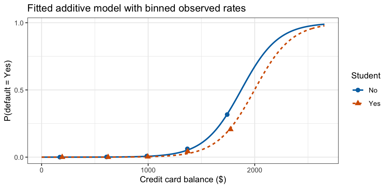

The two curves have the same shape, with the student curve shifted to the right, and both sets of binned points track their own curve. On the log-odds scale the curves are parallel lines separated by $\hat\beta_2$ at every balance; on the probability scale they never cross, and the gap between them closes at both ends. The gap is widest near a balance of $1,936, where it reaches 0.177 in estimated probability — not at the midpoint of the balance range, but where both curves are passing through the steep part of their climb.

A confidence interval for $p(x)$ goes through the same three scales as the one-feature case, with $x$ now a full row of feature values. predict() with type = "link" and se.fit = TRUE returns $\hat\eta(x) = x\hat\beta$ and $\text{SE}(\hat\eta(x))$, giving a Wald interval for the log-odds at $x$; exponentiating both endpoints carries it to an interval for the odds at $x$; and applying $p = \text{odds}/(1+\text{odds})$ to both endpoints of that carries it to an interval for $p(x)$ itself.

x0 <- tibble(balance = 1500,
            student = factor("No", levels = levels(Default$student)))

For a non-student at a balance of $1,500:

link_x0    <- predict(additive_glm, newdata = x0, type = "link", se.fit = TRUE)
eta_hat_x0 <- link_x0$fit
eta_ci_x0  <- eta_hat_x0 + c(-1, 1) * qnorm(0.975) * link_x0$se.fit
odds_ci_x0 <- exp(eta_ci_x0)
p_ci_x0    <- odds_ci_x0 / (1 + odds_ci_x0)

ci_walkthrough <- tibble(
  Scale    = c("Log-odds", "Odds", "P(default)"),
  Estimate = c(eta_hat_x0, exp(eta_hat_x0), plogis(eta_hat_x0)),
  Lower    = c(eta_ci_x0[1], odds_ci_x0[1], p_ci_x0[1]),
  Upper    = c(eta_ci_x0[2], odds_ci_x0[2], p_ci_x0[2])
) |>
  mutate(across(c(Estimate, Lower, Upper), \(x) sprintf("%.4f", x))) |>
  knitr::kable(col.names = c("Scale", "Estimate", "2.5%", "97.5%"),
               align = "lccc")

Scale	Estimate	2.5%	97.5%
Log-odds	-2.1423	-2.3109	-1.9738
Odds	0.1174	0.0992	0.1389
P(default)	0.1050	0.0902	0.1220

Nothing about the three-scale route changed by adding a second feature: $x$ now has three entries instead of two, but $\hat\eta(x)$, its standard error, and the two increasing transforms that follow are exactly what the one-feature lecture used.

10.3 Balance confounds student status

Question. Does being a student change a customer’s risk of default, or does that comparison change once their balances are put on equal footing?

Data. The same 10,000 customers as throughout this lecture, default as the response, with balance and student both as features.

The binned default rates from the exploratory analysis are worth having in view again:

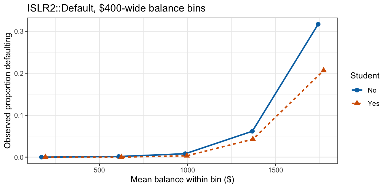
Within every bin the student curve sat at or below the non-student curve, while a student’s balance averaged higher than a non-student’s — the two descriptive facts a model with both features has to reconcile.

10.3.1 Fitting both models

Both fits are already in hand: student_glm, with student alone, and additive_glm, with balance and student together.

Code

fits_comparison <- tibble(
  term = names(ba),
  "Student alone" = c(bs["(Intercept)"], NA, bs["studentYes"]),
  "Balance + student" = ba
) |>
  mutate(across(c("Student alone", "Balance + student"),
                \(x) ifelse(is.na(x), "", sprintf("%.4f", x)))) |>
  knitr::kable(col.names = c("Coefficient", "Student alone",
                             "Balance + student"),
               align = "lcc")

Coefficient	Student alone	Balance + student
(Intercept)	-3.5041	-10.7495
balance		0.0057
studentYes	0.4049	-0.7149

The two intercepts are not comparable: each is the log-odds for a non-student at whatever balance is $0$ in that model, and the student-alone model never holds balance fixed at all.

10.3.2 Fitted probabilities

Each model’s fitted probabilities, against the same binned observed rates used above:

Code

student_newdata <- tibble(student = factor(c("No", "Yes"),
                                           levels = levels(Default$student)))
student_link    <- predict(student_glm, newdata = student_newdata,
                           type = "link", se.fit = TRUE)
student_ci <- student_newdata |>
  mutate(eta   = student_link$fit,
         se    = student_link$se.fit,
         p_hat = plogis(eta),
         lower = plogis(eta - qnorm(0.975) * se),
         upper = plogis(eta + qnorm(0.975) * se))

student_band <- curve_grid |>
  select(balance, student) |>
  left_join(student_ci |> select(student, p_hat, lower, upper), by = "student")

default_prob_base <- ggplot(mapping = aes(x = balance, color = student,
                                          linetype = student)) +
  geom_point(data = binned_rates, aes(y = rate, shape = student, size = n)) +
  coord_cartesian(xlim = c(0, max(Default$balance)), ylim = c(0, 1)) +
  scale_color_manual(values = c("#0072B2", "#D55E00")) +
  scale_size_area(max_size = 5) +
  labs(x = "Credit card balance ($)", y = "P(default = Yes)",
       color = "Student", linetype = "Student", shape = "Student",
       size = "Customers\nin bin", title = "ISLR2::Default")

default_prob_data <- default_prob_base

default_prob_student_alone <- default_prob_base +
  geom_ribbon(data = student_band, aes(ymin = lower, ymax = upper, fill = student),
             color = NA, alpha = 0.2) +
  geom_line(data = student_band, aes(y = p_hat), linewidth = 0.9) +
  scale_fill_manual(values = c("#0072B2", "#D55E00"), guide = "none")

default_prob_balance_fixed <- default_prob_base +
  geom_ribbon(data = curve_grid, aes(ymin = lower, ymax = upper, fill = student),
             color = NA, alpha = 0.2) +
  geom_line(data = curve_grid, aes(y = p_hat), linewidth = 0.9) +
  scale_fill_manual(values = c("#0072B2", "#D55E00"), guide = "none")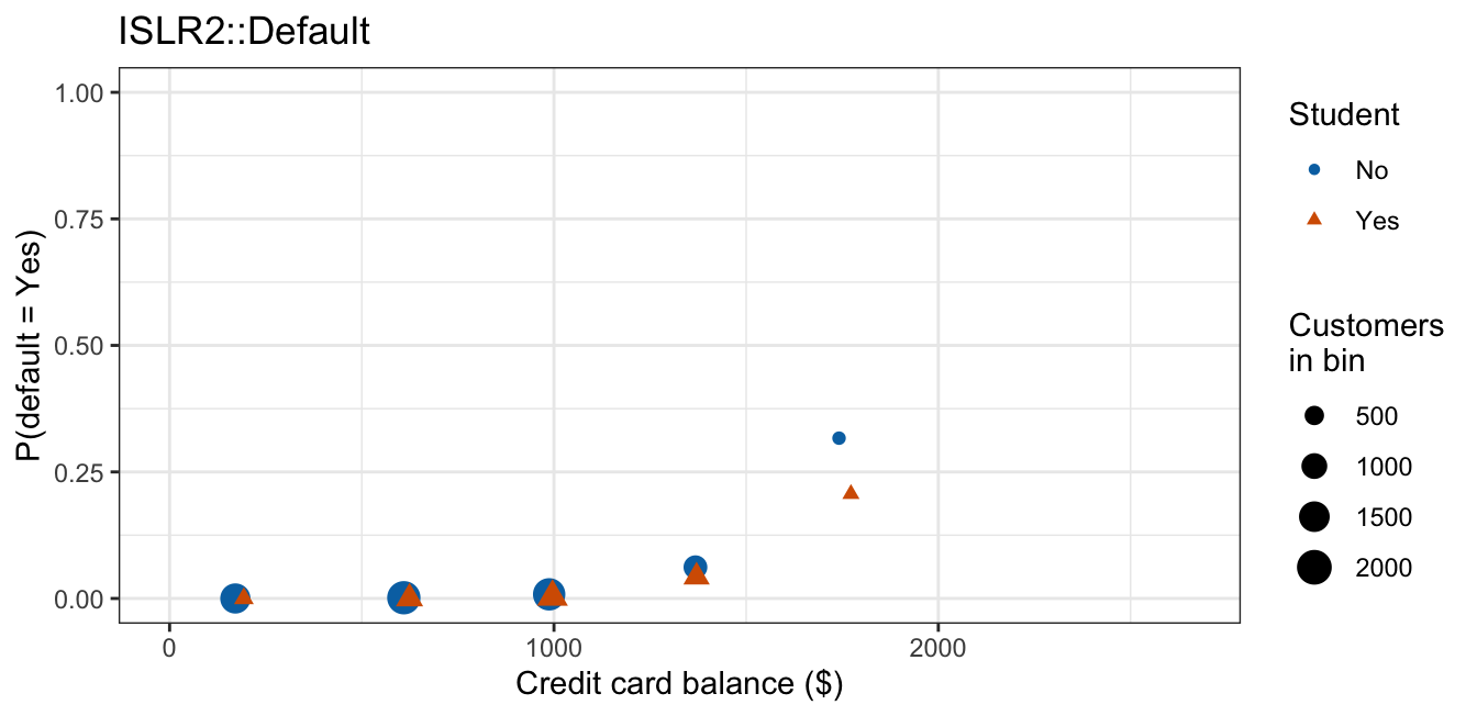

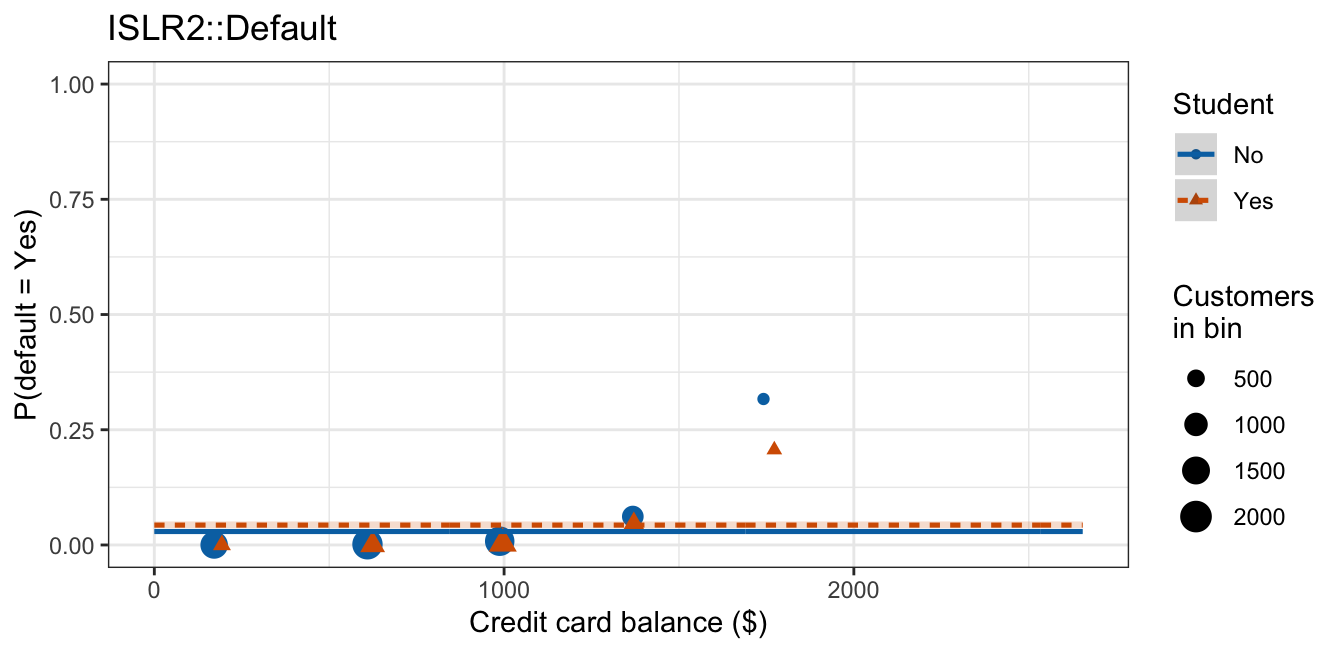
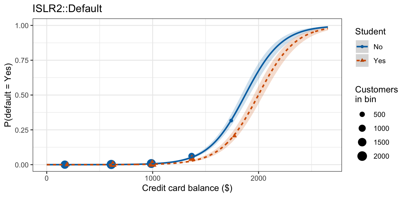
Fit alone, student cannot respond to balance at all — its tab shows two flat lines, and the “Yes” line sits above the “No” line, matching the higher aggregate default rate students showed at the start of this lecture. Once balance is in the model, its tab shows two curves that both climb with balance, and now the “Yes” curve sits below the “No” curve at every balance on the page. The direction of the student effect flips depending on whether balance is held fixed.

10.3.3 Coefficient reversal

Putting the pieces together algebraically, the fitted log-odds are

\[\log\left[\frac{\hat p(X)}{1 - \hat p(X)}\right] = -10.75 +0.005738 \times \texttt{balance} -0.715 \times D.\]

The intercept $\hat\beta_0 = -10.75$ is the estimated log-odds of default for a non-student carrying no balance — both features at zero — which corresponds to an estimated probability of 0.000021.

The other two coefficients are easier to read as odds ratios, with balance rescaled to $100 increments as in the previous lecture:

round(c("balance, per $100" = or_balance_100,
        "student vs. non-student" = or_student_adj), 3)

      balance, per $100 student vs. non-student 
                  1.775                   0.489

Holding student status fixed, an additional $100 of balance multiplies the estimated odds of default by 1.78.

Holding balance fixed, a student’s estimated odds of default are 0.49 times a non-student’s — a 51% reduction in the odds. Fit alone, student status multiplied the odds by 1.50, a 50% increase. The sign of the student coefficient reversed, from $0.405$ to $-0.715$, and nothing about the data changed between the two fits — only which features were held fixed when reading the coefficient.

A marginal association that reverses direction once a third variable is held fixed, at every level of that third variable, is an instance of Simpson’s paradox.

Code

comparison_table <- tibble(
  Model = c("`default ~ student`", "`default ~ balance + student`"),
  Compares = c("a student against a non-student, balances as they happen to be",
               "a student against a non-student **at the same balance**"),
  OR = sprintf("%.2f", c(or_student_alone, or_student_adj))
) |>
  knitr::kable(col.names = c("Model", "What the `student` coefficient compares",
                              "Estimated odds ratio"),
               align = "lll")

Model	What the `student` coefficient compares	Estimated odds ratio
`default ~ student`	a student against a non-student, balances as they happen to be	1.50
`default ~ balance + student`	a student against a non-student at the same balance	0.49

The two descriptive summaries from the exploratory analysis supply the mechanism. Students carry $216 more balance on average, and balance raises the odds of default sharply. A comparison of students to non-students that does not hold balance fixed is therefore partly a comparison of higher balances to lower balances. Once balance is in the model and held fixed, that path is closed, and what remains is the within-balance comparison the binned plot already showed: at a given balance, students default less.

This is confounding: a feature left out of the model is associated both with the feature being interpreted and with the response, so the included feature’s coefficient reports the two associations combined rather than its own. In the one-feature model, student stood in for balance, and the absorbed part was large enough and of the opposite sign to flip the total.

Choosing which coefficient to report

Neither is wrong; they answer different questions, and the question decides.

A credit card company deciding what a new applicant’s student status implies about risk, knowing nothing else about them, wants the one-feature answer: among the customers we see, students default more. A company setting a credit limit for a customer whose balance it already knows wants the additive answer: at that balance, a student is the safer of the two.

What is not defensible is reporting one number and describing it with the other’s interpretation.

10.4 Conclusion

Multiple logistic regression passes multiple linear regression’s linear predictor $\mathbf{X}\beta$ through the logistic function, estimated by the same Bernoulli maximum likelihood as the one-feature case. Each $\beta_j$ is a change in log-odds, and $e^{\beta_j}$ an odds ratio, holding every other feature in the model fixed — the qualifier that distinguishes a coefficient here from the same feature’s coefficient fit alone, and the reason the two can disagree in magnitude or even in sign.

Testing several coefficients at once needs more than a $z$-statistic per coefficient: the drop-in-deviance test compares a reduced and a full model’s residual deviances the way an F-test compares two models’ residual sums of squares, with a $\chi^2$ reference distribution in place of an $F$.

A coefficient’s sign can reverse between a model that omits a feature and one that includes it whenever the omitted feature is associated with both the included feature and the response — confounding, and when the association runs in the opposite direction at every level of the third variable, an instance of Simpson’s paradox. The question being asked decides which comparison — and which coefficient — is the right one to report.

The additive model forces every feature’s odds ratio to be the same regardless of the other features’ values; relaxing that constraint requires interactions between features.