write the multiple regression model in matrix form and derive the least squares estimator \(\hat\beta = (\mathbf{X}^\top \mathbf{X})^{-1}\mathbf{X}^\top y\),
encode a categorical explanatory variable with dummy variables and interpret the resulting coefficients relative to the reference level,
interpret a coefficient and a coefficient on a logged response or explanatory variable,
construct t-tests and confidence intervals for coefficients, and distinguish a confidence interval for the mean response at \(x_0\) from a prediction interval for a new observation, and
conduct an F-test comparing two nested models and explain the F-statistic in terms of the residual sums of squares of the reduced and full models.
where \(f\) is an unknown function and \(\epsilon\) is a random error term with mean 0 and variance \(\sigma^2\). We now consider \(X\) a vector of \(p\) explanatory variables, and we can use a multiple linear regression model to approximate \(f\).
6.1 Multiple explanatory variables
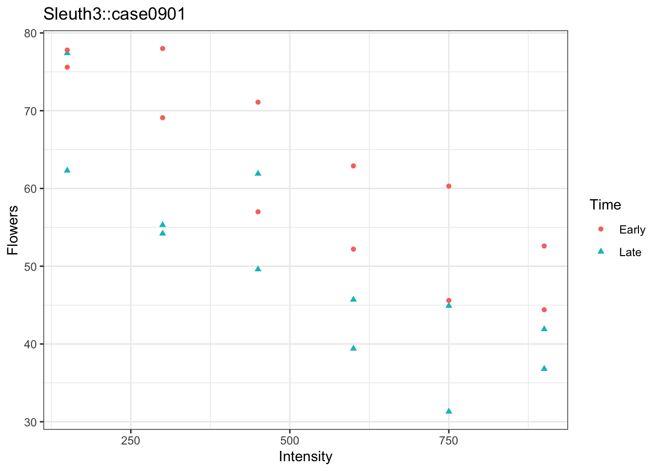
Meadowfoam is grown for the oil in its seed, and how much light the plants get affects how many flowers they produce. In one experiment, plots of meadowfoam were raised under a range of light intensities, with the light begun either early or late in the growing cycle, and the average number of flowers per plant recorded for each plot (Sleuth3::case0901). Two explanatory variables were varied on purpose, so any model of flower production has to account for both of them at once.
d <- Sleuth3::case0901 |>mutate(Time =case_when( Time ==1~"Late", Time ==2~"Early" ))g <-ggplot(d, aes(x = Intensity, y = Flowers, color = Time, shape = Time)) +geom_point() +labs(title ="Sleuth3::case0901")g
Flower production falls as intensity rises, and at nearly every intensity the plots whose light began early out-produced those whose light began late. A model containing intensity alone would have to charge that vertical gap to error, and a model containing timing alone would have to charge the downward trend to error. Multiple regression holds both.
where \(\epsilon_i\) is a random error term with \(E[\epsilon_i] = 0\) and \(Var[\epsilon_i] = \sigma^2\).
Alternatively the model can be written
\[Y = \mathbf{X}\beta + \epsilon\]
where
\(Y = (Y_1, \ldots, Y_n)^\top\) is the vector of responses,
\(\mathbf{X}\) is the \(n \times (p+1)\) model matrix with rows \[X_i = (1, X_{i1}, \ldots, X_{ip})\]
\(\beta = (\beta_0, \ldots, \beta_p)^\top\) is the vector of regression coefficients, and
\(\epsilon = (\epsilon_1, \ldots, \epsilon_n)^\top\) is the vector of random errors.
The error assumptions are now \(E[\epsilon] = 0\) and \(Var[\epsilon] = \sigma^2 I\), where \(I\) is the \(n \times n\) identity matrix.
Throughout we will assume the \(\mathbf{X}\) matrix is of full rank, i.e. \(\mathrm{rank}(\mathbf{X}) = p+1\), but later we will learn about methods such as ridge regression, lasso and principal component regression that can be used when this assumption is violated.
6.3 Categorical explanatory variables
If you have categorical explanatory variables, you can include them in the model using dummy variables. Suppose you have a categorical variable \(Z\) with \(k\) levels. You can create \(k-1\) dummy variables to represent the levels of \(Z\).
For example, if \(Z\) has levels A, B, and C, let’s choose C as the reference level and create two dummy variables for A and B:
Then, you can include these dummy variables in the regression model as follows: \[Y_i = \beta_0 + \beta_1 D_{iA} + \beta_2 D_{iB} + \epsilon_i.\]
6.4 Interpretation
The interpretation of the parameters is as follows:
\(\beta_0\) is the expected response when all explanatory variables are zero and
\(\beta_j\) is the expected change in \(Y\) for a one-unit increase in \(X_j\) when all other explanatory variables are held constant.
When using polynomial terms, e.g. quadratic, or interactions, the interpretation of the coefficients becomes more complex.
NoteInterpretations using logarithms
A common transformation is to take the logarithm of the response variable, the explanatory variable, or both. The interpretations of the parameters change accordingly:
If we take the logarithm of the response variable, then \(e^{\beta_j}\) represents the multiplicative change in the median response for a one-unit increase in the explanatory variable when all other explanatory variables are held constant.
If we take the logarithm of the explanatory variable, then \(\beta_j\log(2)\) represents the expected change in the response for a doubling of the explanatory variable when all other explanatory variables are held constant.
If we take the logarithm of both the response and explanatory variables, then \(2^{\beta_j}\) represents the multiplicative change in the median response for a doubling of the explanatory variable when all other explanatory variables are held constant.
NoteBeyond this course
Another tool that helps interpretation of models is the use of contrasts. Contrasts are linear combinations of the regression coefficients that allow us to test specific hypotheses about the relationships between the explanatory variables and the response variable.
6.5 Estimation
The vector \(\beta = (\beta_0, \beta_1, \ldots, \beta_p)^\top\) is estimated using the method of least squares:
For inference, we need to assume normality of the errors, i.e. \[\epsilon_i \stackrel{ind}{\sim} N(0, \sigma^2).\] This results in the model \[Y_i \stackrel{ind}{\sim} N(\beta_0 + \beta_1 X_{i1}+\cdots+\beta_pX_{ip}, \sigma^2)\] or, equivalently,
\[Y \sim N_n(\mathbf{X}\beta, \sigma^2 I)\] where \(N_n\) is the \(n\)-dimensional multivariate normal distribution.
With the normality assumption, we can write the likelihood function:
the estimates for \(\beta\) that maximize this likelihood are the same as those obtained from least squares. These are referred to as the maximum likelihood estimators (MLEs) of \(\beta\).
6.6.1 t-tests
For testing hypotheses about the regression coefficients, we use t-tests. The test statistic for \(\beta_j\) is
where \(t_{n-(p+1), 1-\alpha/2}\) is the \((1-\alpha/2)\) quantile of the t-distribution with \(n-(p+1)\) degrees of freedom.
The standard error of \(\hat{\beta}_j\) is given by \[\text{SE}\left(\hat{\beta}_j\right) = \sqrt{\hat{\sigma}^2 \left(\mathbf{X}^\top \mathbf{X}\right)^{-1}_{jj}}\] where \(\left(\mathbf{X}^\top \mathbf{X}\right)^{-1}_{jj}\) is the \(j\)-th diagonal element of the inverse of the matrix \(\mathbf{X}^\top \mathbf{X}\).
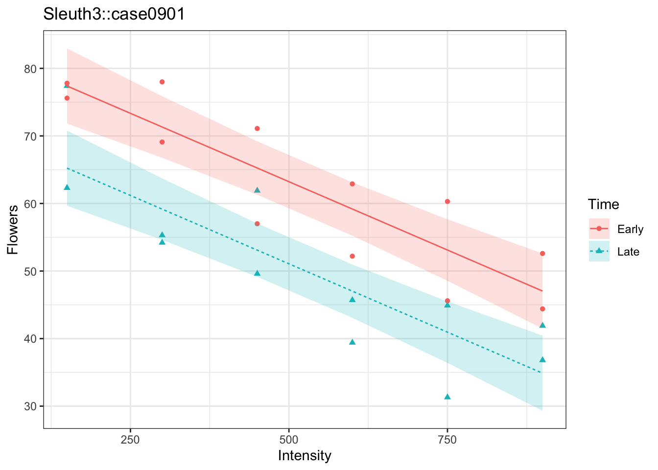
where \(x_0\) is now a vector of feature values, \(\hat{f}(x_0) = x_0^\top\hat\beta = \hat{\beta}_0 + \hat{\beta}_1 x_{01} + \cdots + \hat\beta_p x_{0p}\), and \(\text{SE}(\hat{f}(x_0))\) is the standard error of the predicted mean response. This is the uncertainty in the line at a given point \(x_0\).
nd <-unique(d |>select(Intensity, Time))cx <-bind_cols(nd, predict( m, newdata =unique(d |>select(Intensity, Time)), interval ="confidence", level =0.95)) |>rename(Flowers = fit )cx
   Intensity  Time  Flowers      lwr      upr
1        150  Late 65.23512 59.66986 70.80038
2        300  Late 59.16440 54.61256 63.71625
3        450  Late 53.09369 49.14491 57.04247
4        600  Late 47.02298 43.07420 50.97175
5        750  Late 40.95226 36.40042 45.50410
6        900  Late 34.88155 29.31629 40.44681
7        150 Early 77.39345 71.82819 82.95871
8        300 Early 71.32274 66.77090 75.87458
9        450 Early 65.25202 61.30325 69.20080
10       600 Early 59.18131 55.23253 63.13009
11       750 Early 53.11060 48.55875 57.66244
12       900 Early 47.03988 41.47462 52.60514
g +geom_ribbon(data = cx, aes(ymin = lwr, ymax = upr, fill = Time), color =NA, alpha =0.2) +geom_line(data = cx, aes(linetype = Time))
6.7 Prediction
A \((1-\alpha)100\%\) prediction interval for a new observation at a specific value \(x_0\) is given by \[\hat{Y}_0 \pm t_{n-(p+1), 1-\alpha/2} \cdot \text{SE}_{\text{pred}}(\hat{Y}_0)\]
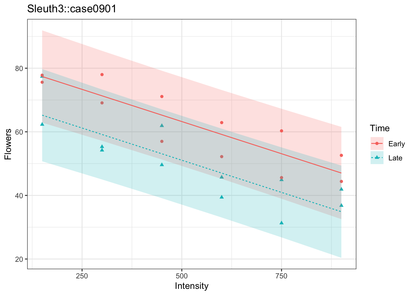
where \(\hat{Y}_0 = \hat{f}(x_0) = x_0^\top\hat\beta\) and \(\text{SE}_{\text{pred}}(\hat{Y}_0)\) is the standard error of the predicted value, which accounts for both the uncertainty in the mean response and the variability of individual observations. The key here is that the prediction interval is wider than the confidence interval for the mean response, reflecting the additional uncertainty in predicting a single new observation due to the residual error \(\epsilon\).
px <-bind_cols(nd, predict( m, newdata =unique(d |>select(Intensity, Time)), interval ="prediction", # THIS CHANGEDlevel =0.95)) |>rename(Flowers = fit )px
   Intensity  Time  Flowers      lwr      upr
1        150  Late 65.23512 50.73006 79.74017
2        300  Late 59.16440 45.01719 73.31162
3        450  Late 53.09369 39.12883 67.05855
4        600  Late 47.02298 33.05811 60.98784
5        750  Late 40.95226 26.80504 55.09948
6        900  Late 34.88155 20.37649 49.38660
7        150 Early 77.39345 62.88840 91.89851
8        300 Early 71.32274 57.17552 85.46996
9        450 Early 65.25202 51.28716 79.21689
10       600 Early 59.18131 45.21645 73.14617
11       750 Early 53.11060 38.96338 67.25781
12       900 Early 47.03988 32.53483 61.54494
g +geom_ribbon(data = px, aes(ymin = lwr, ymax = upr, fill = Time), color =NA, alpha =0.2) +geom_line(data = px, aes(linetype = Time))
6.8 F-tests
To evaluate the statistical evidence for a group of explanatory variables, e.g. a single categorical variable with \(k+1\) levels, we can use an F-test. The null hypothesis is that all coefficients for the group of variables are equal to zero, i.e \[H_0: \beta_{j_1} = \beta_{j_2} = \cdots = \beta_{j_k} = 0\] where \(j_1, j_2, \ldots, j_k\) are the indices of the coefficients for the group of variables. The alternative hypothesis is that at least one of the coefficients is not equal to zero. The F-statistic is calculated as \[F_{k, n-(p+1)}
= \frac{(RSS_r - RSS_f)/k}{RSS_f/(n-[p+1])}
= \frac{(RSS_r - RSS_f)/k}{\hat\sigma^2_{f}}\]
where
\(RSS_r\) is the residual sum of squares for the reduced model (without the group of variables),
\(RSS_f\) is the residual sum of squares for the full model (with the group of variables),
\(k\) is the difference in the number of coefficients between the two models, and
\(n-(p+1)\) is the degrees of freedom for the full model.
Under the null hypothesis, the F-statistic follows an F-distribution with \(k\) and \(n-(p+1)\) degrees of freedom. A \(p\)-value can be calculated from the F-distribution to assess the statistical significance of the group of variables.
# Defaultanova(m)
Analysis of Variance Table

Response: Flowers
          Df  Sum Sq Mean Sq F value    Pr(>F)
Intensity  1 2579.75 2579.75  62.181 1.037e-07 ***
Time       1  886.95  886.95  21.379 0.0001464 ***
Residuals 21  871.24   41.49
---
Signif. codes:  0 '***' 0.001 '**' 0.01 '*' 0.05 '.' 0.1 ' ' 1
drop1(m, test="F")
Single term deletions

Model:
Flowers ~ Intensity + Time
          Df Sum of Sq    RSS     AIC F value    Pr(>F)
<none>                  871.2  92.205
Intensity  1   2579.75 3451.0 123.241  62.181 1.037e-07 ***
Time       1    886.95 1758.2 107.056  21.379 0.0001464 ***
---
Signif. codes:  0 '***' 0.001 '**' 0.01 '*' 0.05 '.' 0.1 ' ' 1
tail(capture.output(summary(m)), n =2)[1]
[1] "F-statistic: 41.78 on 2 and 21 DF, p-value: 4.786e-08"
# Manual (for nested models)m0 <-lm(Flowers ~1, data = d) # Intercept only modelanova(m0, m)
Analysis of Variance Table

Model 1: Flowers ~ 1
Model 2: Flowers ~ Intensity + Time
  Res.Df    RSS Df Sum of Sq     F    Pr(>F)
1     23 4337.9
2     21  871.2  2    3466.7 41.78 4.786e-08 ***
---
Signif. codes:  0 '***' 0.001 '**' 0.01 '*' 0.05 '.' 0.1 ' ' 1
6.9 Model Assessment
6.9.1 R-squared
The coefficient of determination, \(R^2\), measures the proportion of the variance in the response variable that is predictable from the explanatory variable(s). It is defined as \[R^2 = 1 - \frac{RSS}{TSS}\]
where \(RSS\) is the residual sum of squares and \(TSS\) is the total sum of squares, i.e.
\[TSS = \sum_{i=1}^n (y_i - \bar{y})^2.\]
Thus, \(R^2\) can be interpreted as the proportion of the total variability in the response variable that is explained by the model.
summary(m)$r.squared
[1] 0.7991589
6.10 Meadowfoam flower production
Collecting the pieces above into one analysis: does light intensity change the number of flowers a meadowfoam plant produces, and does the timing of the light matter once intensity is accounted for?
The experiment varied intensity over 6 levels and timing over 2, with 2 plots at each combination and 24 plots in all, so the design is balanced and neither explanatory variable can stand in for the other. Before fitting the model, look at the data with a separate least squares line through each timing group:
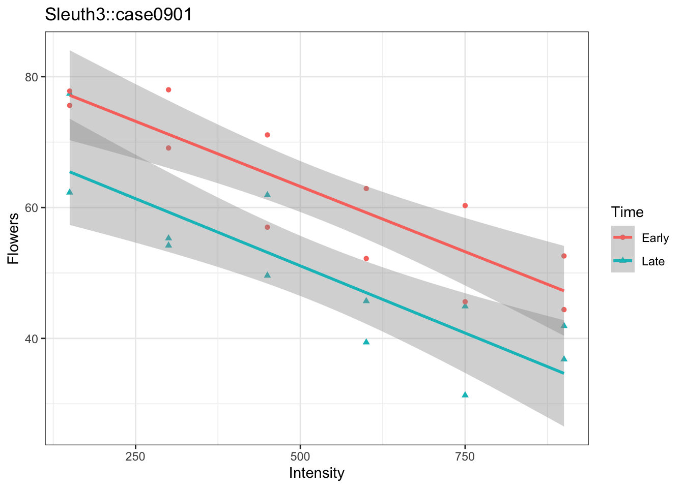
g +geom_smooth(method ="lm", formula = y ~ x)
Both groups trend downward at a similar rate, with the early group’s line sitting above the late group’s across the whole range of intensity. The two slopes are close enough that a model forcing them to be equal — one slope on intensity, plus a constant vertical shift for timing — looks like a reasonable description of these data.
That model is the additive fit m from above, Flowers ~ Intensity + Time:
summary(m)
Call:
lm(formula = Flowers ~ Intensity + Time, data = d)

Residuals:
   Min     1Q Median     3Q    Max
-9.652 -4.139 -1.558  5.632 12.165

Coefficients:
              Estimate Std. Error t value Pr(>|t|)
(Intercept)  83.464167   3.273772  25.495  < 2e-16 ***
Intensity    -0.040471   0.005132  -7.886 1.04e-07 ***
TimeLate    -12.158333   2.629557  -4.624 0.000146 ***
---
Signif. codes:  0 '***' 0.001 '**' 0.01 '*' 0.05 '.' 0.1 ' ' 1

Residual standard error: 6.441 on 21 degrees of freedom
Multiple R-squared:  0.7992,    Adjusted R-squared:   0.78
F-statistic: 41.78 on 2 and 21 DF,  p-value: 4.786e-08
Read the coefficients in order.
\(\hat\beta_0 = 83.5\) is the expected number of flowers at zero intensity for the reference timing, which R takes to be Early because it orders the levels alphabetically. Zero light lies outside the observed intensity range of 150 to 900 μmol/m²/sec, so the intercept anchors the fitted lines rather than predicting a realizable condition.
\(\hat\beta_1 = -0.0405\) says that each additional μmol/m²/sec of light is associated with 0.0405 fewer flowers, holding timing fixed. Over the 150 units separating consecutive intensities in the design, that is 6.1 fewer flowers.
\(\hat\beta_2 = -12.2\) is the coefficient on the dummy variable for Late, so plots whose light began late produced that many fewer flowers than plots at the same intensity whose light began early. Its 95% confidence interval, \((-17.6,
-6.7)\), excludes zero.
The F-test against the intercept-only model gives \(F = 41.8\) on \(2\) and \(21\) degrees of freedom, and the two explanatory variables together account for \(R^2 = 80\%\) of the variability in flower counts.
Both explanatory variables earn their place: flower production declines with intensity, and at any fixed intensity beginning the light early is worth about 12 additional flowers per plant. The one assumption the data have not been asked about is the parallel-lines restriction the additive model imposes — that the slope on intensity is the same for both timings.
6.11 Conclusion
Multiple linear regression writes the mean response as a linear combination of \(p\) explanatory variables, \(Y_i = \beta_0 + \beta_1X_{i1} + \cdots + \beta_pX_{ip} + \epsilon_i\), or in matrix form \(Y = \mathbf{X}\beta + \epsilon\). Least squares gives \(\hat\beta = (\mathbf{X}^\top\mathbf{X})^{-1}\mathbf{X}^\top y\) whenever \(\mathbf{X}\) has full rank, the normal-error likelihood makes that same vector the maximum likelihood estimator, and the error variance is estimated by \(\hat\sigma^2 = RSS/[n - (p+1)]\), one degree of freedom spent per estimated coefficient.
A categorical explanatory variable with \(k\) levels enters through \(k-1\) dummy variables defined against a reference level: the intercept absorbs the reference level, and each dummy’s coefficient is a difference from it. Every coefficient in the model, dummy or not, now carries the qualifier holding the other explanatory variables fixed, which is what separates it from the coefficient the same variable would get in a regression by itself.
Inference divides by the question. A t-test and a confidence interval speak about one coefficient; a confidence interval for the mean response at \(x_0\) speaks about where the fitted surface is; a prediction interval speaks about where a new observation will fall and is wider by that observation’s own error variance. Testing several coefficients at once — every dummy from one categorical variable, say — requires the F-test, which compares the residual sums of squares of a reduced and a full model and asks whether the drop is larger than the extra parameters can explain by chance.
Next lecture keeps this model and the estimator derived for it, but stops requiring the columns of \(\mathbf{X}\) to be the raw explanatory variables. Polynomials and interactions are features built from those variables, and because the model stays linear in \(\beta\), everything above carries over unchanged.