library("tidyverse")
library("quantmod")

theme_set(theme_bw())

# ------------------------------------------------------------------------------
# Get data
# ------------------------------------------------------------------------------

# Define date range
start_date <- "2000-01-01"
end_date <- Sys.Date()

# Download Equity data from Yahoo Finance
getSymbols("AAPL", from = start_date, to = end_date, auto.assign = TRUE)
getSymbols("SPY", from = start_date, to = end_date, auto.assign = TRUE)
getSymbols("^IRX", from = start_date, to = end_date, auto.assign = TRUE) # 13-Week T-Bill Yield Index

# Calculate weekly returns for equity tickers
aapl_weekly <- weeklyReturn(AAPL, type = "arithmetic")
spy_weekly <- weeklyReturn(SPY, type = "arithmetic")

# Process the T-Bill (^IRX) data
# Extract the closing yield values matching our equity weekly date index
# Using Ad() gets the adjusted close, or Cl() for regular close
t_bill_weekly_yield <- Cl(IRX)[index(spy_weekly)]

# Forward-fill any missing data gap days (like market holidays)
t_bill_weekly_yield <- na.locf(t_bill_weekly_yield, na.rm = TRUE)

# Convert annualized yield percentage to weekly decimal: (Yield / 100) / 52
t_bill_weekly_return <- (t_bill_weekly_yield / 100) / 52

# Merge all series into one object and rename columns
merged_returns <- merge(aapl_weekly, spy_weekly, t_bill_weekly_return)
colnames(merged_returns) <- c(
  "AAPL_Return",
  "SPY_Return",
  "TBill_Weekly_Yield"
)

# Convert the xts object to a standard data.frame
d <- data.frame(Date = index(merged_returns), coredata(merged_returns)) |>
  na.omit() |>
  remove_rownames() |>
  mutate(
    AAPL_Excess_Return = AAPL_Return - TBill_Weekly_Yield,
    SPY_Excess_Return = SPY_Return - TBill_Weekly_Yield
  )

# ------------------------------------------------------------------------------
# Exploratory Data Analysis (EDA)
# ------------------------------------------------------------------------------

scatter_plot <- ggplot(d, aes(x = SPY_Excess_Return, y = AAPL_Excess_Return)) +
  geom_point(alpha = 0.5) +
  labs(
    title = "Scatter Plot of AAPL vs SPY Weekly Returns",
    x = "SPY Weekly Excess Return",
    y = "AAPL Weekly Excess Return"
  )

scatter_plot

# Hexbin plot
hexbin_plot <- ggplot(d, aes(x = SPY_Excess_Return, y = AAPL_Excess_Return)) +
  geom_hex(bins = 30) +
  labs(
    title = "Hexbin Plot of AAPL vs SPY Weekly Returns",
    x = "SPY Weekly Excess Return",
    y = "AAPL Weekly Excess Return"
  ) +
  scale_fill_gradient(low = "lightblue", high = "darkblue")

hexbin_plot

hexbin_smooth_plot <- hexbin_plot + geom_smooth(method = "lm", formula = y ~ x)
hexbin_smooth_plot

# ------------------------------------------------------------------------------
# Fit the CAPM model using simple linear regression
# ------------------------------------------------------------------------------

# Fit the linear regression model: AAPL excess return ~ SPY excess return
capm_model <- lm(AAPL_Excess_Return ~ SPY_Excess_Return, data = d)

# View the summary of the CAPM model
summary(capm_model)

coef(capm_model)
confint(capm_model)
summary(capm_model)$r.squared5 Capital Asset Pricing Model
TipLearning objectives
After this lecture you should be able to
- derive the CAPM regression equation from the CAPM formula,
- interpret the intercept and slope of the fitted regression in financial terms, i.e. excess return and beta,
- fit the CAPM model in R using weekly returns downloaded from Yahoo Finance, and
- evaluate a fitted CAPM model by comparing its \(R^2\) and estimated beta to those of another asset.
The Capital Asset Pricing Model (CAPM) is a widely used model in finance that describes the relationship between systematic risk and expected return for assets, particularly stocks. The CAPM formula is given by: \[E[R] = R_f + \beta (E[R_m] - R_f)\] where
- \(R\) is the return of the asset,
- \(R_f\) is the risk-free rate, and
- \(R_m\) is the return of the market portfolio.
The return of the asset is calculated based on the current and previous price of the asset. If the price at time \(t\) is \(P_t\) and the price at time \(t-1\) is \(P_{t-1}\), then the return of the asset at time \(t\) is given by: \[R_t = \frac{P_t - P_{t-1}}{P_{t-1}}.\]
To fit a simple linear regression model to the CAPM, we can rewrite the equation in the form of a linear regression model: \[\underbrace{R_t - R_{t,f}}_{\text{response}} = \beta_0 + \beta_1 \underbrace{(R_{t,m} - R_{t,f})}_{\text{explanatory}} + \epsilon_t\] where, at time \(t\),
- \(R_t\) is the asset return,
- \(R_{t,f}\) is the risk-free return, and
- \(R_{t,m}\) is the market return.
Taking expectations of both sides and substituting the CAPM formula for \(E[R_t]\) and \(E[R_{t,m}]\),
\[E[R_t - R_{t,f}] = \beta_1 (E[R_{t,m}] - R_{t,f}),\]
which matches the regression equation above only if \(\beta_0 = 0\). CAPM is therefore making a testable prediction about the intercept, not just the slope.
The coefficient interpretations in this model are
- \(\beta_0\) is the asset’s abnormal return, or alpha — the part of its excess return not explained by market exposure. CAPM implies \(\beta_0 = 0\), so an estimate far from zero is evidence against the model, and
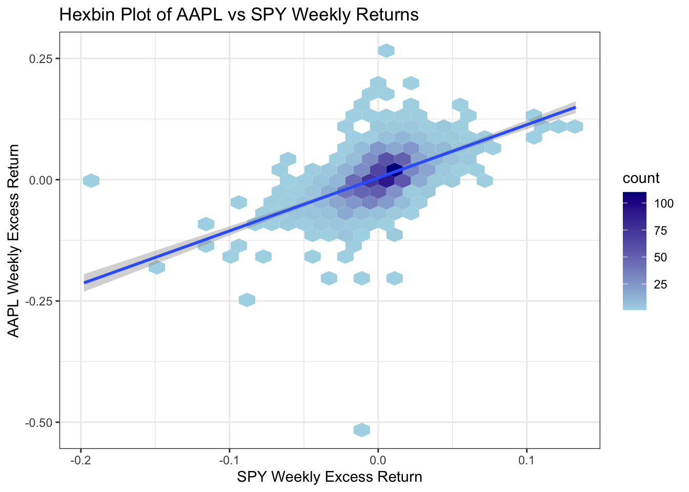
- \(\beta_1\) is the asset’s sensitivity to market movements, also known as the asset’s beta.
5.1 Apple against the S&P 500
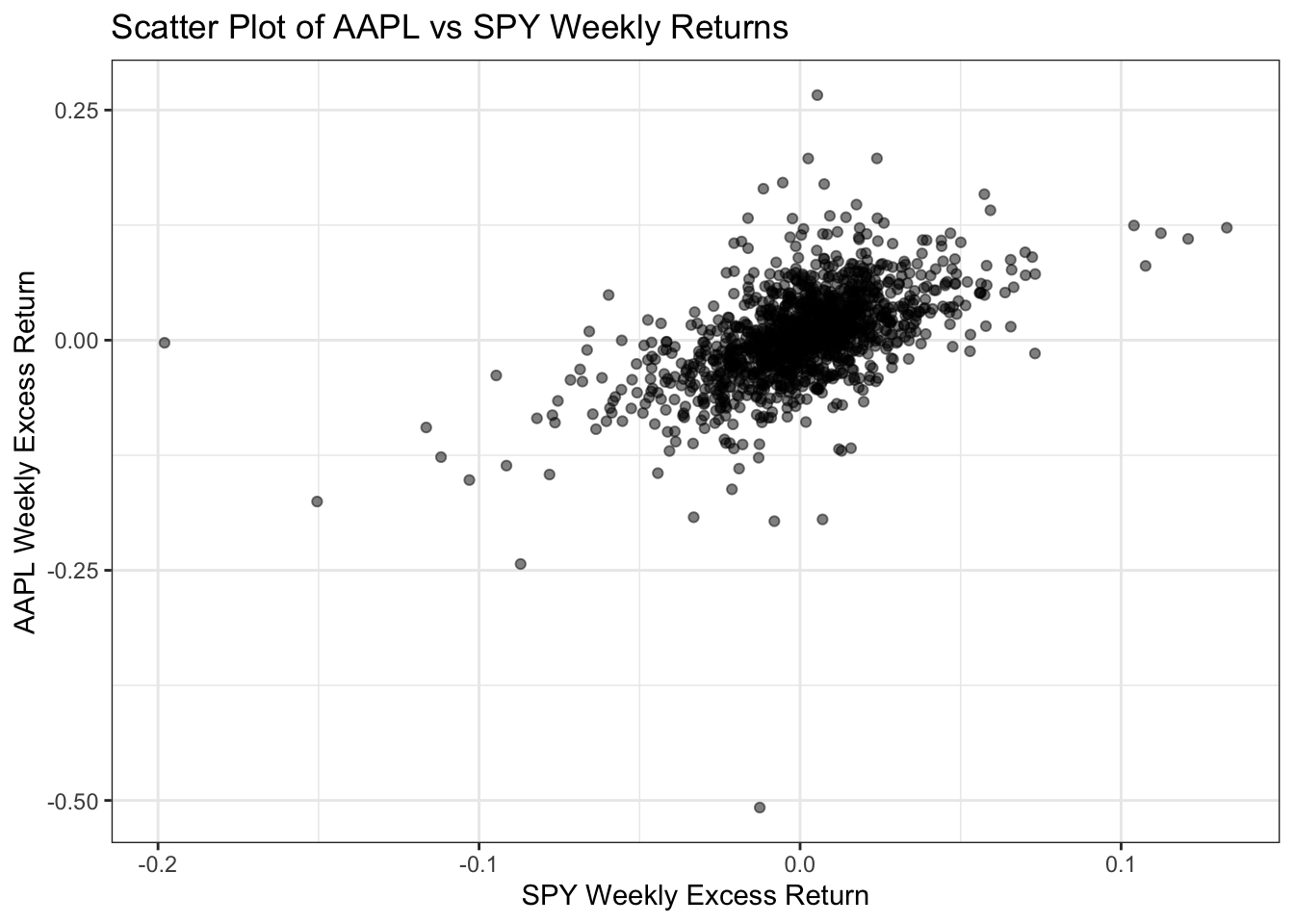
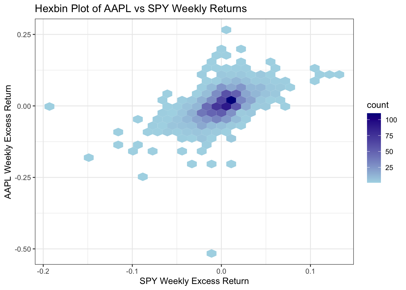
We fit the CAPM using Apple (AAPL) as the asset, the S&P 500 ETF (SPY) as the market portfolio, and the 13-week T-bill yield (^IRX) as the risk-free rate.
NoteCode
Call:
lm(formula = AAPL_Excess_Return ~ SPY_Excess_Return, data = d)

Residuals:
     Min       1Q   Median       3Q      Max
-0.49795 -0.02050 -0.00154  0.02130  0.25640

Coefficients:
                  Estimate Std. Error t value Pr(>|t|)
(Intercept)       0.003948   0.001135   3.478  0.00052 ***
SPY_Excess_Return 1.094636   0.046181  23.703  < 2e-16 ***
---
Signif. codes:  0 '***' 0.001 '**' 0.01 '*' 0.05 '.' 0.1 ' ' 1

Residual standard error: 0.04235 on 1393 degrees of freedom
Multiple R-squared:  0.2874,    Adjusted R-squared:  0.2869
F-statistic: 561.8 on 1 and 1393 DF,  p-value: < 2.2e-16
(Intercept) SPY_Excess_Return
0.003947991 1.094635805 2.5 % 97.5 %
(Intercept) 0.001721342 0.006174641
SPY_Excess_Return 1.004044344 1.185227266[1] 0.28741135.2 Class activity
Find a stock, or an index, whose CAPM fit against SPY has
- a higher \(R^2\) than AAPL’s, and
- a more extreme beta, i.e. farther from 1 in either direction, than AAPL’s.
Adapt the code above by substituting your chosen ticker for AAPL (getSymbols() accepts any Yahoo Finance ticker), re-fit the model, and report the resulting \(R^2\) and \(\hat\beta_1\) alongside AAPL’s for comparison.
5.3 Conclusion
CAPM is a financial model, but subtracting the risk-free rate from both the asset’s return and the market’s turns it into a simple linear regression of one excess return on the other. Once the model is in that form, lm() fits it, confint() gives intervals for its coefficients, and summary() reports \(R^2\), with no new estimation theory required.
The finance lives in the interpretation. The intercept \(\beta_0\) is the asset’s alpha, the expected excess return left over when the market is flat, and CAPM predicts it is exactly zero — an unusual situation in which theory names a specific null value for an intercept, so the t-test already printed in the regression output is a test of the model itself. The slope \(\beta_1\) is the asset’s beta, the expected change in its excess return for a one-unit change in the market’s, so a beta above one amplifies market movements and a beta below one damps them. \(R^2\) measures how much of the asset’s excess return moves with the market at all: a fund holding the index would sit near one, a single company well below it, and the unexplained remainder is the asset’s idiosyncratic risk — the part of its variability that diversification can remove.
A large beta says the asset is sensitive to the market, not that it earns more: both coefficients describe an association between two contemporaneous excess returns, estimated over the particular window of history the downloaded data cover.
Next lecture extends the model from one explanatory variable to several. The same reasoning that produced CAPM produces multi-factor models, which regress an asset’s excess return on the market’s and on additional explanatory variables, and multiple regression is the machinery for fitting and testing them.