17 Cross-Validation

Learning objectives

After this lecture you should be able to

explain why training error cannot choose a model’s flexibility, and identify the two weaknesses of the validation set approach: its estimate varies from one random split to the next, and it overestimates the test error of a model fit to all \(n\) observations,
define the leave-one-out and \(k\)-fold cross-validation estimates of test MSE and test error rate, and implement each as a loop that fits on all but one fold and predicts the held-out fold,
derive the least squares shortcut \(\text{CV}_{(n)} = \frac{1}{n}\sum_{i=1}^n\left[\left(y_i - \hat y_i\right)/\left(1 - h_i\right)\right]^2\) and interpret the role of the leverage \(h_i\) in it,
compare the validation set approach, leave-one-out, and \(k\)-fold cross-validation by the bias and variance of their test-error estimates and by computation, and justify the usual choice \(k = 5\) or \(10\),
use cross-validation to choose a flexibility setting, such as a polynomial degree or the number of neighbors \(K\) in KNN, and
identify the data-dependent steps of a fit (feature screening, standardization) that must be repeated inside every fold, and explain why performing them once on all the data makes the cross-validation estimate optimistic.

17.1 Test error estimation

17.1.1 Horsepower and fuel efficiency

Question. How flexible should a regression of a car’s fuel efficiency on its engine horsepower be?

Data. ISLR2::Auto records 392 cars. The response is mpg, miles per gallon, and the explanatory variable is horsepower. The figure plots one against the other.

Code

auto_base <- ggplot(Auto, aes(x = horsepower, y = mpg)) +
  geom_point(alpha = 0.4, size = 1) +
  coord_cartesian(ylim = range(Auto$mpg)) +
  labs(x = "Horsepower", y = "Miles per gallon", title = "ISLR2::Auto")

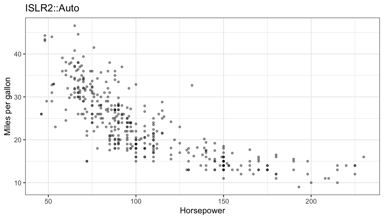
Fuel efficiency falls as horsepower rises, steeply at first and then more slowly.

Model. To follow that curvature, the candidate models are polynomial regressions of degree \(d\),

\[\texttt{mpg}_i = \beta_0 + \beta_1\,\texttt{horsepower}_i + \beta_2\,\texttt{horsepower}_i^2 + \cdots + \beta_d\,\texttt{horsepower}_i^d + \epsilon_i, \qquad \epsilon_i \stackrel{ind}{\sim} N\left(0, \sigma^2\right),\]

where

\(\texttt{mpg}_i\) and \(\texttt{horsepower}_i\) are the fuel efficiency and horsepower of car \(i = 1, \ldots, n\),
\(d\) is the degree of the polynomial, the flexibility setting to be chosen,
\(\beta_0, \ldots, \beta_d\) are the coefficients and \(\epsilon_i\) the error, with variance \(\sigma^2\), and
the features are the \(d\) powers of horsepower, so row \(i\) of the model matrix \(\mathbf{X}\) is \(x_i = \left(1, \texttt{horsepower}_i, \ldots, \texttt{horsepower}_i^d\right)\).

As in the feature engineering lecture, poly(horsepower, d) fits the same model with an orthogonal basis of the same column space, so its fitted values are identical.

Code

degrees <- 1:10
show_degrees <- c(1, 2, 10)
degree_labels <- paste("Degree", show_degrees)
degree_colors <- setNames(c("#0072B2", "#D55E00", "#009E73"), degree_labels)
degree_linetypes <- setNames(c("solid", "dashed", "dotdash"), degree_labels)

hp_grid <- tibble(horsepower = seq(min(Auto$horsepower), max(Auto$horsepower),
                                   length.out = 400))
degree_curves <- map(show_degrees, \(d) {
  fit <- lm(mpg ~ poly(horsepower, d), data = Auto)
  mutate(hp_grid, degree = paste("Degree", d), mpg = predict(fit, hp_grid))
}) |>
  list_rbind() |>
  mutate(degree = factor(degree, levels = degree_labels))

add_curves <- function(through) {
  auto_base +
    geom_line(data = filter(degree_curves, as.integer(degree) <= through),
              aes(color = degree, linetype = degree), linewidth = 1) +
    scale_color_manual(values = degree_colors) +
    scale_linetype_manual(values = degree_linetypes) +
    labs(color = "Polynomial", linetype = "Polynomial")
}
auto_curve_plots <- map(seq_along(show_degrees), add_curves)

The tabs add least squares fits of degree 1, 2, and 10 to the plot above.

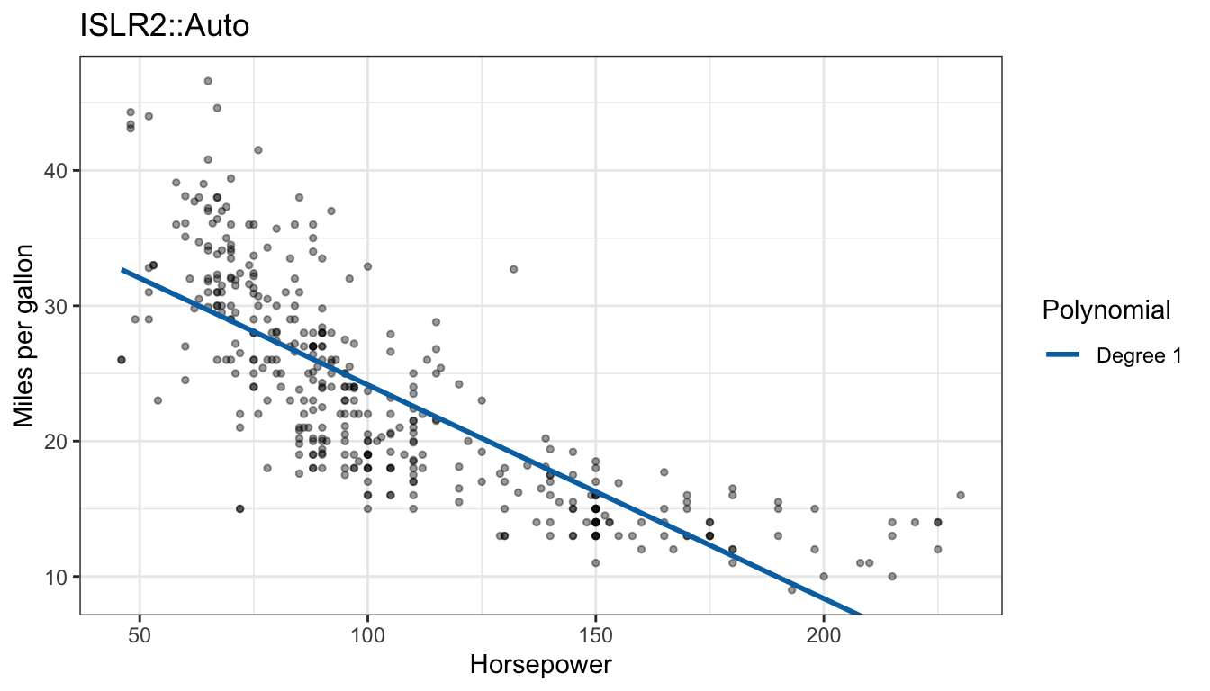
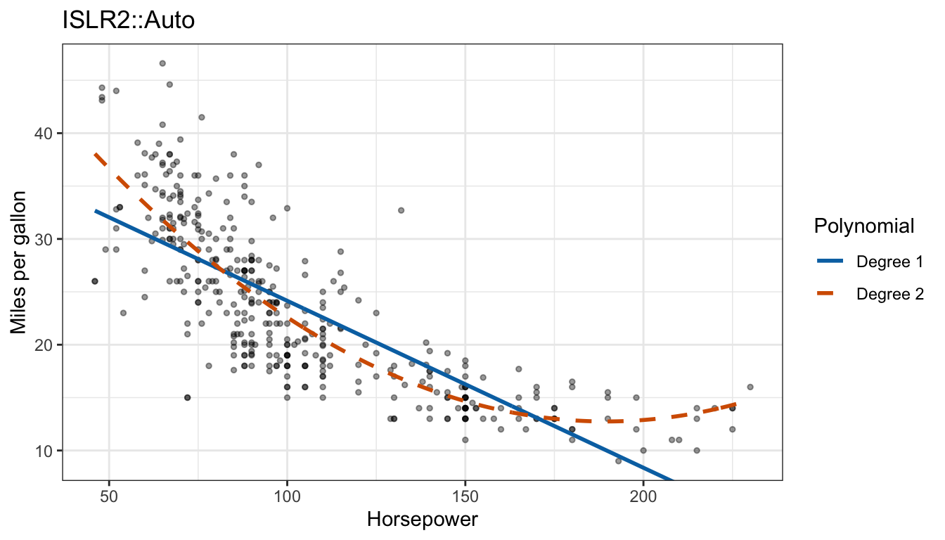
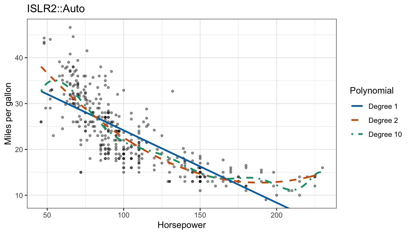
The straight line misses the curvature: it underpredicts at both ends and overpredicts in the middle. The quadratic follows the curve. The degree-10 polynomial follows it too, with extra wiggles at both ends of the range of horsepower, where cars are few.

17.1.2 Training MSE

The function below fits a degree-\(d\) polynomial to a data set; applied to all 392 cars it gives the training MSE of each degree.

fit_degree <- function(d, data) lm(mpg ~ poly(horsepower, d), data = data)
train_mse <- map_dbl(degrees, \(d) mean(residuals(fit_degree(d, Auto))^2))

Code

train_mse_plot <- ggplot(tibble(degree = degrees, mse = train_mse),
                         aes(x = degree, y = mse)) +
  geom_line() +
  geom_point() +
  scale_x_continuous(breaks = degrees) +
  labs(x = "Polynomial degree d", y = "Training MSE", title = "ISLR2::Auto")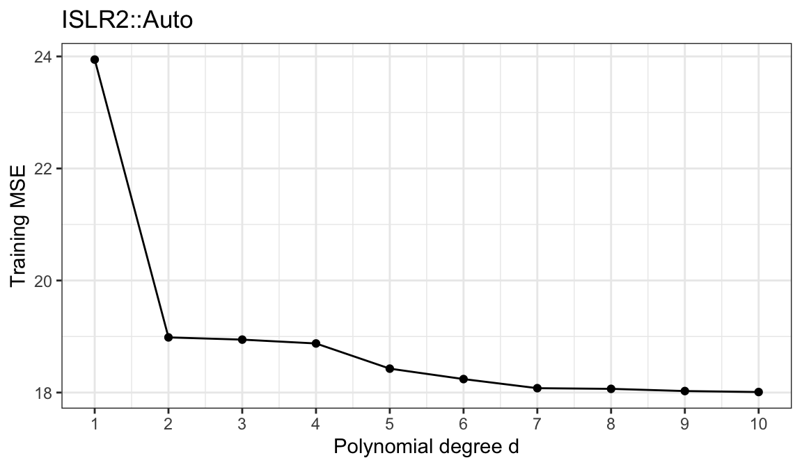

The training MSE falls from 23.94 at degree 1 to 18.98 at degree 2 and keeps falling, to 18.01 at degree 10. It cannot do otherwise: the degree-\(d\) model is the degree-\((d+1)\) model with \(\beta_{d+1} = 0\), so least squares over the larger model can only match or lower the residual sum of squares. Training error rewards flexibility whether or not the flexibility captures anything that will appear in new data, so it cannot choose \(d\).

17.1.3 Held-out data

The regression lecture defined the test MSE as the average squared error on observations that were not used to estimate \(\hat f\). With a large, separate set of data held out from fitting, choosing \(d\) would be easy: fit each degree to the training data and keep the degree with the smallest test MSE. A separate test set is rarely available. Collecting one costs as much as collecting the training data, and setting aside part of the data already in hand leaves less to fit with.

Resampling methods estimate test error from the training data alone, by fitting the model to part of the data and measuring its error on the part left out. This lecture develops three, in increasing order of reuse: the validation set approach, leave-one-out cross-validation, and \(k\)-fold cross-validation.

The data play three different roles, and the names keep them apart. The training set is what a model is fit to. A validation set, such as the held-out part in the next section or a held-out fold in cross-validation, is part of the data in hand that was held out from fitting; its prediction error estimates the test error and is used to compare models and choose tuning parameters such as \(d\). Test data are observations that were never used to fit a model or to choose among models, so only they give an estimate of the test error that the choosing has not affected.

17.2 Validation set approach

The figure below shows the cars split at random into two halves of 196, a training set (blue circles) and a validation set (orange triangles).

Code

n_auto <- nrow(Auto)
n_splits <- 100
splits <- map(seq_len(n_splits), \(r) sample(n_auto, n_auto / 2))
one_split <- splits[[1]]

set_colors <- c(Training = "#0072B2", Validation = "#E69F00")
split_plot <- Auto |>
  mutate(set = if_else(row_number() %in% one_split, "Training", "Validation")) |>
  ggplot(aes(x = horsepower, y = mpg, color = set, shape = set)) +
  geom_point(alpha = 0.7, size = 1.3) +
  scale_color_manual(values = set_colors) +
  scale_shape_manual(values = c(Training = 16, Validation = 17)) +
  labs(x = "Horsepower", y = "Miles per gallon", color = NULL, shape = NULL,
       title = "ISLR2::Auto, one random split")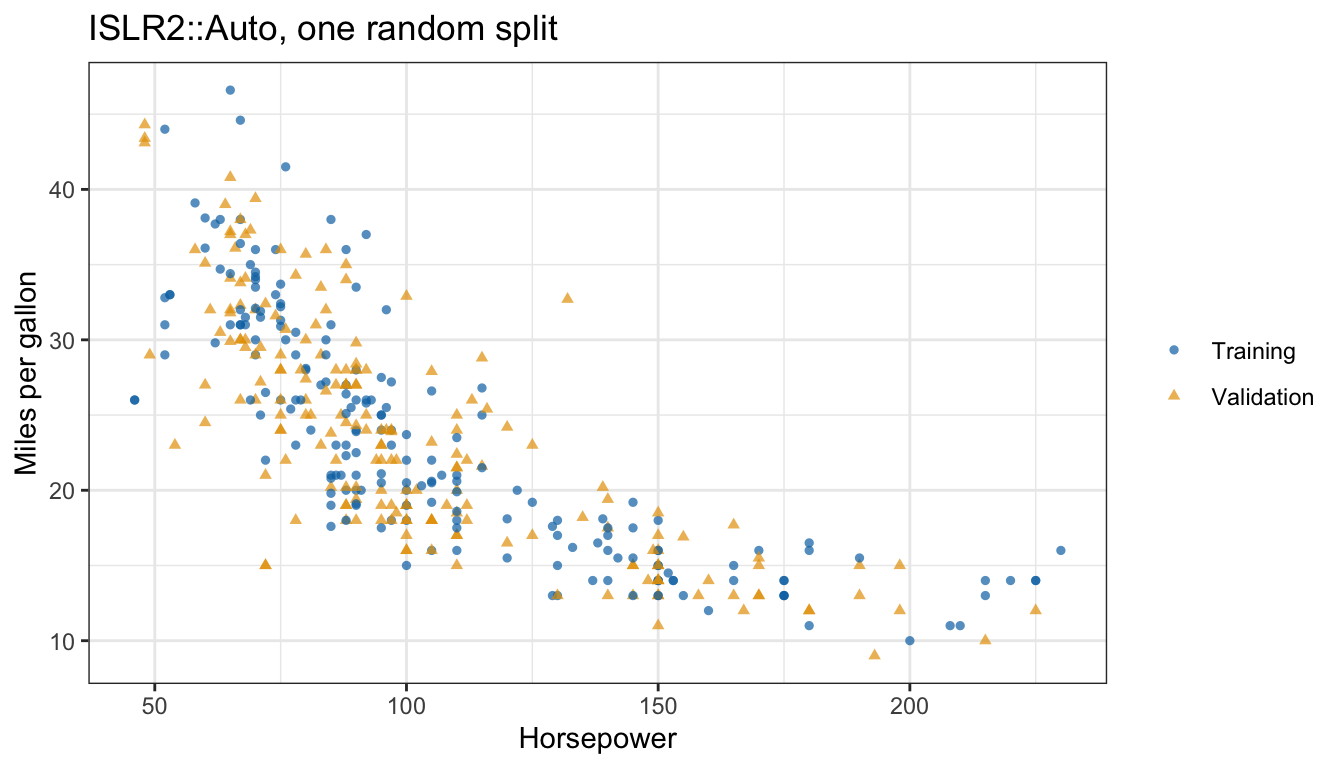

Both halves cover the range of horsepower, and either half shows the same curved decline as the full data.

17.2.1 Algorithm

The validation set approach estimates test MSE in three steps:

Split the \(n\) observations at random into a training set and a validation (hold-out) set \(\mathcal{V}\).
Fit the model to the training set.
Predict every observation in the validation set and average the squared errors,

\[\text{MSE}_{\mathcal{V}} = \frac{1}{n_{\mathcal{V}}}\sum_{i \in \mathcal{V}}\left[y_i - \hat f(x_i)\right]^2,\]

where

\(\mathcal{V}\) is the set of indices of the validation observations and \(n_{\mathcal{V}}\) their number, and
\(\hat f\) is the model fit to the training set only.

Every validation observation is new to \(\hat f\), so \(\text{MSE}_{\mathcal{V}}\) estimates the test MSE. It is also used to choose among degrees, so the validation set is not untouched test data. In R, with train_id the row numbers of the training set:

validation_mse <- function(d, train_id, data = Auto) {
  fit <- fit_degree(d, data[train_id, ])
  valid <- data[-train_id, ]
  mean((valid$mpg - predict(fit, valid))^2)
}
one_split_mse <- map_dbl(degrees, validation_mse, train_id = one_split)

17.2.2 Split variability

The split above is one of 100 random splits into halves. The first tab plots its validation MSE against degree, the second adds the curves of all 100 splits (grey, with the first in black), and the third counts the degree with the smallest validation MSE in each split.

Code

val_curves <- expand_grid(split = seq_len(n_splits), degree = degrees) |>
  mutate(mse = map2_dbl(degree, split, \(d, r) validation_mse(d, splits[[r]])))
val_best <- val_curves |>
  group_by(split) |>
  slice_min(mse, n = 1, with_ties = FALSE) |>
  ungroup()
val_choice_counts <- count(val_best, degree)
val_mse_d2 <- filter(val_curves, degree == 2)$mse
# Within each split, the spread of the estimates over degrees 2 through 10.
within_split_range <- val_curves |>
  filter(degree >= 2) |>
  group_by(split) |>
  summarize(range = max(mse) - min(mse), .groups = "drop")

mse_limits <- c(14, 30)
n_off_plot <- n_distinct(filter(val_curves, mse > mse_limits[2])$split)
degree_axis <- list(scale_x_continuous(breaks = degrees),
                    coord_cartesian(ylim = mse_limits))
one_split_plot <- ggplot(tibble(degree = degrees, mse = one_split_mse),
                         aes(x = degree, y = mse)) +
  geom_line() +
  geom_point() +
  degree_axis +
  labs(x = "Polynomial degree d", y = "Validation MSE",
       title = "One random split into halves")
all_splits_plot <- ggplot(val_curves, aes(x = degree, y = mse, group = split)) +
  geom_line(color = "grey70", linewidth = 0.3) +
  geom_line(data = filter(val_curves, split == 1), color = "black") +
  geom_point(data = filter(val_curves, split == 1), color = "black") +
  degree_axis +
  labs(x = "Polynomial degree d", y = "Validation MSE",
       title = paste(n_splits, "random splits into halves"))
choice_plot <- ggplot(val_best, aes(x = factor(degree, levels = degrees))) +
  geom_bar() +
  scale_x_discrete(drop = FALSE) +
  labs(x = "Degree with the smallest validation MSE", y = "Number of splits",
       title = paste(n_splits, "random splits into halves"))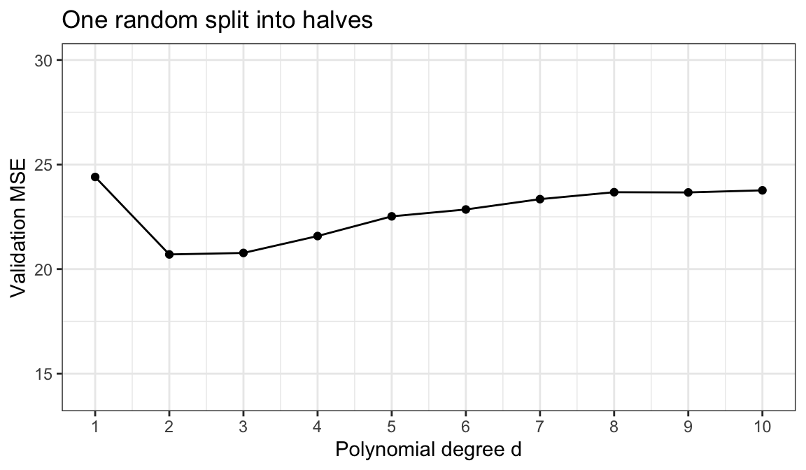

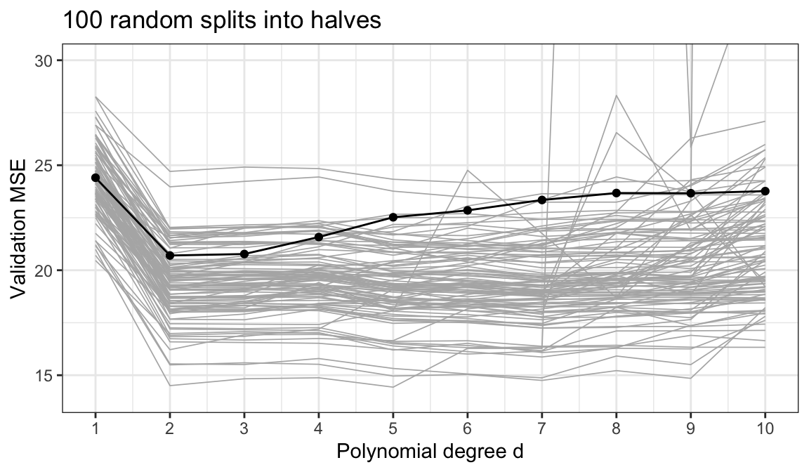
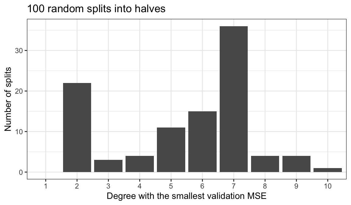
Every curve drops sharply from degree 1 to degree 2, so every split agrees that a quadratic beats a line. Beyond that the splits disagree. The validation MSE of the quadratic ranges from 14.50 to 24.71 across splits, while within a split the estimates for degrees 2 through 10 span a median of 1.87. Of the 100 curves, 2 leave the top of the plot at high degree, where a polynomial fit to half the cars extrapolates badly to a validation car outside their range of horsepower. The degree with the smallest validation MSE is 2, 3, 4, 5, 6, 7, 8, 9, and 10 in different splits; the most common choice, degree 7, wins only 36 of the 100 splits.

This is the first weakness of the validation set approach: the estimate, and the model it selects, depend on which observations happen to land in which half.

17.2.3 Smaller training sets

The second weakness is that each model is fit to only part of the data.

Code

train_sizes <- c(60, 80, 120, 160, n_auto / 2, 240, 280, 320, 360)
learning_degrees <- c(2, 7)
n_learning_reps <- 400
learning <- expand_grid(m = train_sizes, degree = learning_degrees,
                        rep = seq_len(n_learning_reps)) |>
  mutate(mse = map2_dbl(m, degree, \(m, d) validation_mse(d, sample(n_auto, m))))
learning_summary <- learning |>
  group_by(m, degree) |>
  summarize(median_mse = median(mse), mean_mse = mean(mse), .groups = "drop") |>
  mutate(degree = factor(paste("Degree", degree),
                         levels = paste("Degree", learning_degrees)))
learning_of <- function(m_value, d, col = "median_mse") {
  learning_summary[[col]][learning_summary$m == m_value &
                            learning_summary$degree == paste("Degree", d)]
}

learning_plot <- ggplot(learning_summary,
                        aes(x = m, y = median_mse, color = degree,
                            linetype = degree, shape = degree)) +
  geom_vline(xintercept = n_auto / 2, color = "grey60") +
  geom_line() +
  geom_point(size = 2) +
  scale_color_manual(values = c("#0072B2", "#D55E00")) +
  labs(x = "Training set size m (vertical line: half of the cars)",
       y = "Median validation MSE", color = NULL, linetype = NULL,
       shape = NULL, title = paste(n_learning_reps, "random splits at each m"))

To see what that costs, the cars were split at random into a training set of \(m\) cars and a validation set of the remaining \(n - m\), for \(m\) from 60 to 360, 400 times at each \(m\). Because the validation cars are new to each fit, the typical validation MSE at a given \(m\) estimates the test MSE of a model fit to \(m\) cars. The figure plots the median over splits for degrees 2 and 7.

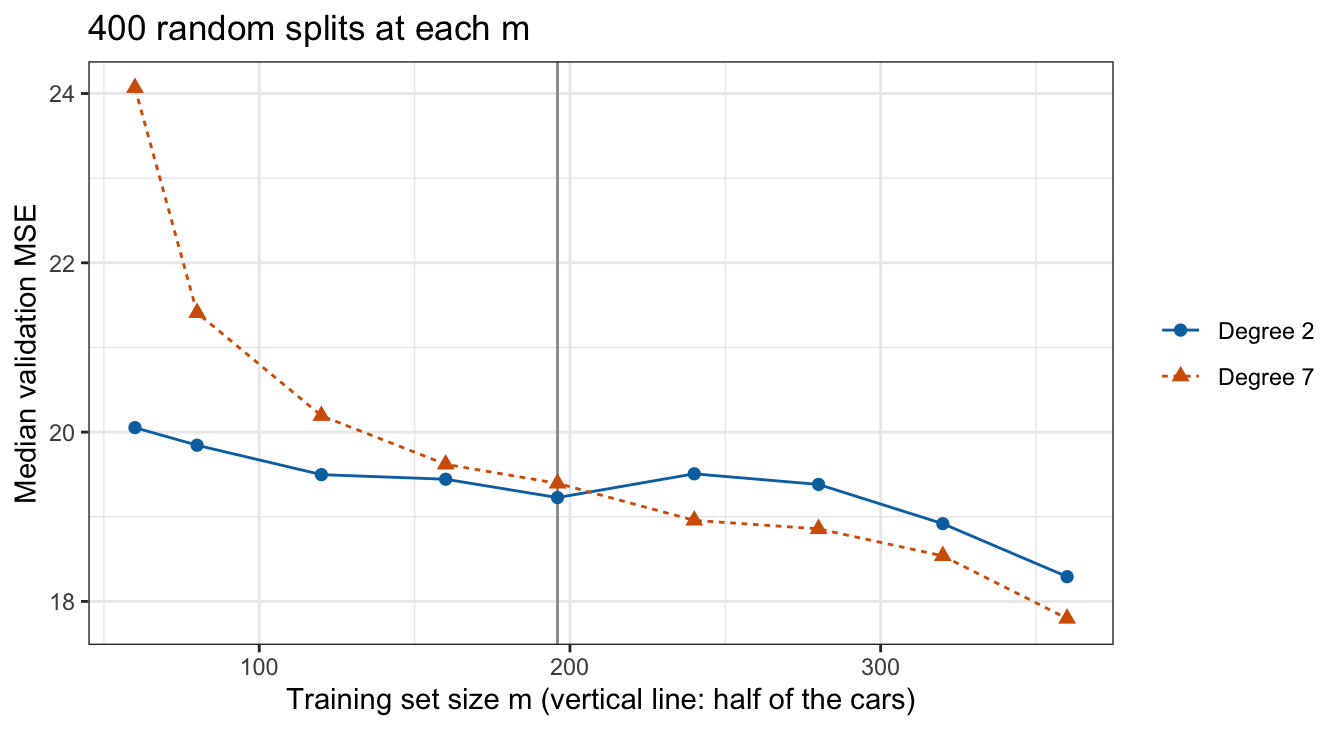
Test MSE generally falls as the training set grows, and it falls more steeply for the more flexible model. The degree-7 polynomial has a median validation MSE of 24.07 when fit to 60 cars, against 19.39 when fit to 196; the quadratic goes from 20.05 to 19.23. (The median is plotted because the mean is dominated by a few catastrophic extrapolations: at \(m = 60\) the mean validation MSE of degree 7 is 5,778.) The model that will be used is fit to all 392 cars, so a validation set estimate computed from fits to half of them estimates the error of a worse model. The validation set approach tends to overestimate the test error of the final fit, and more so for flexible models and small \(n\).

17.3 Leave-one-out cross-validation

The validation set approach leaves out half the data. Leave-one-out cross-validation leaves out one observation at a time. The figure below holds out the car with the largest horsepower, a Pontiac Grand Prix with 230 horsepower (black triangle), and draws the fit to all 392 cars (dashed) and the fit to the other 391 (solid), for degree 2 in the first tab and degree 10 in the second.

Code

i_out <- which.max(Auto$horsepower)
held_out_summary <- map(c(2, 10), \(d) {
  fit_all <- fit_degree(d, Auto)
  fit_without <- fit_degree(d, Auto[-i_out, ])
  tibble(degree = d,
         residual = Auto$mpg[i_out] - fitted(fit_all)[[i_out]],
         loo_error = Auto$mpg[i_out] - predict(fit_without, Auto[i_out, ]),
         leverage = hatvalues(fit_all)[[i_out]])
}) |>
  list_rbind()
held_of <- function(d, col) held_out_summary[[col]][held_out_summary$degree == d]

fit_labels <- c("All cars", "Car held out")
held_out_plot <- function(d) {
  curves <- bind_rows(
    mutate(hp_grid, fit = fit_labels[1],
           mpg = predict(fit_degree(d, Auto), hp_grid)),
    mutate(hp_grid, fit = fit_labels[2],
           mpg = predict(fit_degree(d, Auto[-i_out, ]), hp_grid))) |>
    mutate(fit = factor(fit, levels = fit_labels))
  ggplot(Auto, aes(x = horsepower, y = mpg)) +
    geom_point(data = Auto[-i_out, ], color = "grey60", alpha = 0.5, size = 1) +
    geom_line(data = curves, aes(color = fit, linetype = fit), linewidth = 0.9) +
    geom_point(data = Auto[i_out, ], shape = 17, size = 3.5) +
    scale_color_manual(values = c("#0072B2", "#D55E00")) +
    scale_linetype_manual(values = c("dashed", "solid")) +
    coord_cartesian(ylim = range(Auto$mpg)) +
    labs(x = "Horsepower", y = "Miles per gallon", color = "Fit to",
         linetype = "Fit to", title = paste("Degree", d))
}
held_out_plots <- map(c(2, 10), held_out_plot)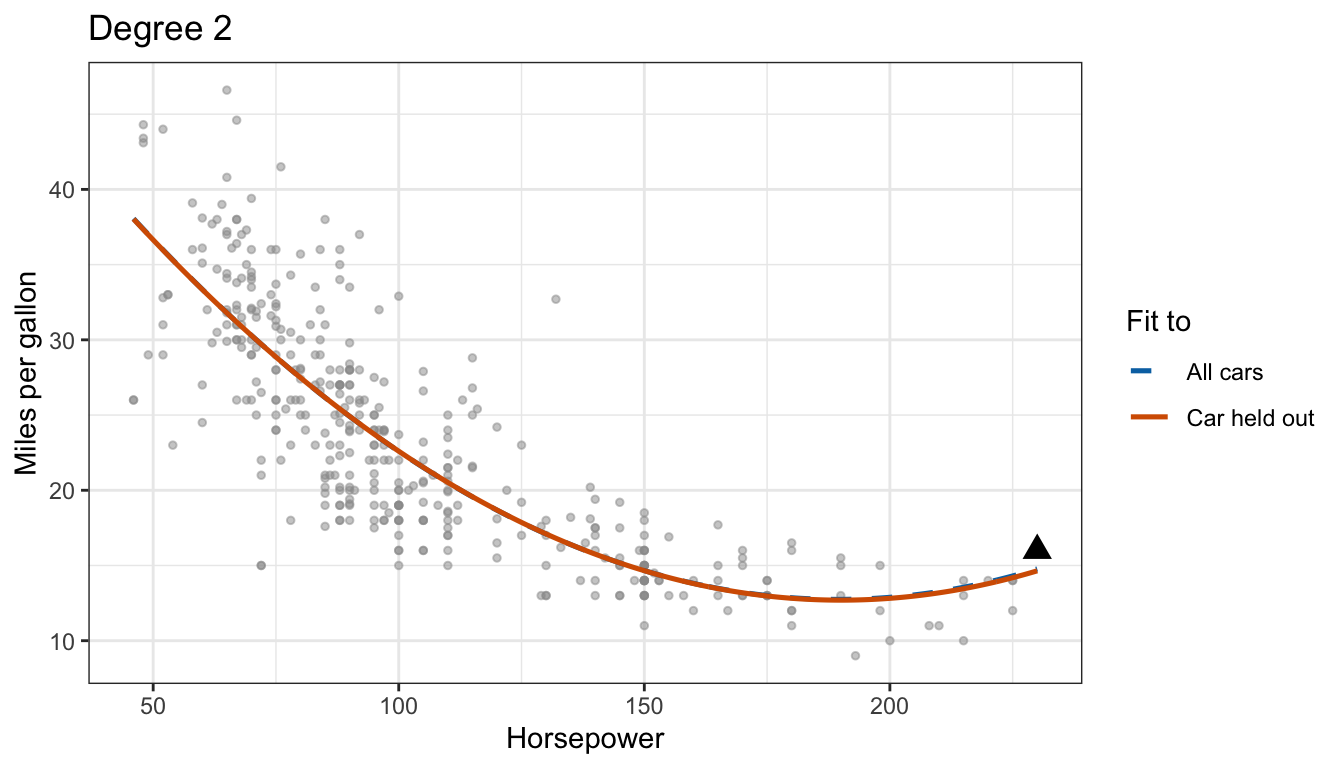

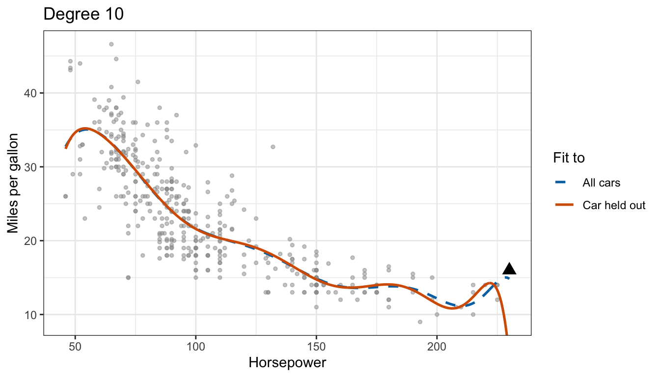
For the quadratic the two fits nearly coincide, and the held-out car is predicted about as well without it as with it. For degree 10 the fit to all cars bends to pass near the held-out car, and without it the curve swings far below. The squared error of the held-out prediction measures how well the model predicts a car it has not seen, which the residual from the fit to all cars does not.

17.3.1 LOOCV estimate

Leave-one-out cross-validation (LOOCV) repeats that for every observation:

\[\text{CV}_{(n)} = \frac{1}{n}\sum_{i=1}^n\left[y_i - \hat f^{(-i)}(x_i)\right]^2,\]

where

\(\hat f^{(-i)}\) is the model fit to the \(n - 1\) observations other than observation \(i\), and
\(\hat f^{(-i)}(x_i)\) is its prediction for the held-out observation.

Each fit uses \(n - 1\) observations, nearly all of the data, and there is no random split: every observation is held out exactly once. Written as a loop, LOOCV costs \(n\) fits per model.

loocv_mse <- function(d, data = Auto) {
  sq_error <- numeric(nrow(data))
  for (i in seq_len(nrow(data))) {
    fit <- fit_degree(d, data[-i, ])
    sq_error[i] <- (data$mpg[i] - predict(fit, data[i, ]))^2
  }
  mean(sq_error)
}
loocv_loop <- map_dbl(degrees, loocv_mse)

17.3.2 Least squares shortcut

For a model fit by least squares, the \(n\) fits are unnecessary. Write the least squares fit to all \(n\) observations as \(\hat y = \mathbf{H}y\), with

\[\mathbf{H} = \mathbf{X}\left(\mathbf{X}^\top\mathbf{X}\right)^{-1}\mathbf{X}^\top, \qquad \hat y_i = \sum_{j=1}^n h_{ij}\,y_j, \qquad h_i = h_{ii} = x_i\left(\mathbf{X}^\top\mathbf{X}\right)^{-1}x_i^\top,\]

where

\(\mathbf{H}\) is the hat matrix and \(h_{ij}\) its \((i, j)\) entry,
\(\hat y_i = x_i\hat\beta\) is the fitted value of observation \(i\) from the fit to all \(n\) observations, and
\(h_i\) is the leverage of observation \(i\), as in the flexibility lecture, with \(0 \le h_i \le 1\).

Let \(\hat\beta^{(-i)}\) be the least squares estimate without observation \(i\), so \(\hat f^{(-i)}(x_i) = x_i\hat\beta^{(-i)}\), and assume \(\mathbf{X}\) without row \(i\) still has full column rank so that \(\hat\beta^{(-i)}\) is unique.

Step 1: a full-data fit that reproduces \(\hat\beta^{(-i)}\). Define a response vector \(z\) equal to \(y\) except in entry \(i\), which is replaced by the held-out prediction: \(z_j = y_j\) for \(j \ne i\) and \(z_i = x_i\hat\beta^{(-i)}\). For any \(\beta\),

\[\sum_{j=1}^n\left(z_j - x_j\beta\right)^2 = \sum_{j \ne i}\left(y_j - x_j\beta\right)^2 + \left(x_i\hat\beta^{(-i)} - x_i\beta\right)^2.\]

The first sum is minimized at \(\beta = \hat\beta^{(-i)}\), by definition, and the second term is zero there, its smallest possible value. So \(\hat\beta^{(-i)}\) minimizes the left side: it is the least squares estimate for response \(z\) with all \(n\) rows, \(\hat\beta^{(-i)} = \left(\mathbf{X}^\top\mathbf{X}\right)^{-1}\mathbf{X}^\top z\).

Step 2: apply the hat matrix. Multiplying by \(x_i\), \(x_i\hat\beta^{(-i)}\) is entry \(i\) of \(\mathbf{H}z\):

\[\hat f^{(-i)}(x_i) = \sum_{j=1}^n h_{ij}\,z_j = \sum_{j=1}^n h_{ij}\,y_j - h_i\,y_i + h_i\,\hat f^{(-i)}(x_i) = \hat y_i - h_i\,y_i + h_i\,\hat f^{(-i)}(x_i).\]

Step 3: solve. Collecting the \(\hat f^{(-i)}(x_i)\) terms, \(\left(1 - h_i\right)\hat f^{(-i)}(x_i) = \hat y_i - h_i y_i\). The full-rank assumption on \(\mathbf{X}\) without row \(i\) makes \(h_i < 1\), so dividing by \(1 - h_i\),

\[y_i - \hat f^{(-i)}(x_i) = \frac{\left(1 - h_i\right)y_i - \hat y_i + h_i y_i}{1 - h_i} = \frac{y_i - \hat y_i}{1 - h_i}.\]

Squaring and averaging over \(i\),

\[\text{CV}_{(n)} = \frac{1}{n}\sum_{i=1}^n\left(\frac{y_i - \hat y_i}{1 - h_i}\right)^2.\]

The held-out error is the ordinary residual inflated by \(1/(1 - h_i)\). With \(h_i = 0\) for every \(i\) this would be the training MSE. The inflation is small for a typical observation and large for a high-leverage one, whose fitted value the full-data fit pulls toward its own response. The formula needs one fit, its residuals, and hatvalues(). It holds for any model fit by least squares on fixed features: polynomials, interactions, step functions with fixed cut points. It does not hold for logistic regression or KNN, where LOOCV takes \(n\) fits.

For the held-out car in the figure, the quadratic gives leverage \(h_i = 0.0936\), residual \(y_i - \hat y_i = 1.228\), and signed held-out error \(y_i - \hat f^{(-i)}(x_i) = 1.35\); the degree-10 polynomial gives leverage \(h_i = 0.9018\), residual 1.168, and signed held-out error 11.90, which equals \(1.168/(1 - 0.9018)\) up to rounding.

The shortcut for every degree:

loocv_shortcut <- function(d, data = Auto) {
  fit <- fit_degree(d, data)
  mean(((data$mpg - fitted(fit)) / (1 - hatvalues(fit)))^2)
}
loocv_fast <- map_dbl(degrees, loocv_shortcut)

Code

loocv_table <- tibble(degree = degrees,
                      loop = fmt(loocv_loop, 4),
                      shortcut = fmt(loocv_fast, 4)) |>
  knitr::kable(col.names = c("Degree $d$",
                             paste0("Loop (", n_auto, " fits)"),
                             "Shortcut (1 fit)"),
               align = "ccc")
max_loocv_diff <- max(abs(loocv_loop - loocv_fast))

Degree \(d\)	Loop (392 fits)	Shortcut (1 fit)
1	24.2315	24.2315
2	19.2482	19.2482
3	19.3350	19.3350
4	19.4244	19.4244
5	19.0332	19.0332
6	18.9786	18.9786
7	18.8330	18.8330
8	18.9612	18.9612
9	19.0686	19.0686
10	19.4909	19.4909

The two columns agree to the digits shown; the largest absolute difference is \(3.0 \times 10^{-12}\), rounding error. The loop needed 3,920 least squares fits and the shortcut 10.

17.3.3 Degree selection

The figure below plots the LOOCV estimate and the training MSE against degree.

Code

loocv_best <- degrees[which.min(loocv_fast)]
error_labels <- c("Training MSE", "LOOCV")
loocv_curve_data <- bind_rows(
  tibble(degree = degrees, mse = train_mse, estimate = error_labels[1]),
  tibble(degree = degrees, mse = loocv_fast, estimate = error_labels[2])) |>
  mutate(estimate = factor(estimate, levels = error_labels))
loocv_curve_plot <- ggplot(loocv_curve_data,
                           aes(x = degree, y = mse, color = estimate,
                               linetype = estimate, shape = estimate)) +
  geom_line() +
  geom_point(size = 2) +
  scale_x_continuous(breaks = degrees) +
  scale_color_manual(values = c("grey40", "#D55E00")) +
  labs(x = "Polynomial degree d", y = "MSE", color = NULL, linetype = NULL,
       shape = NULL, title = "ISLR2::Auto")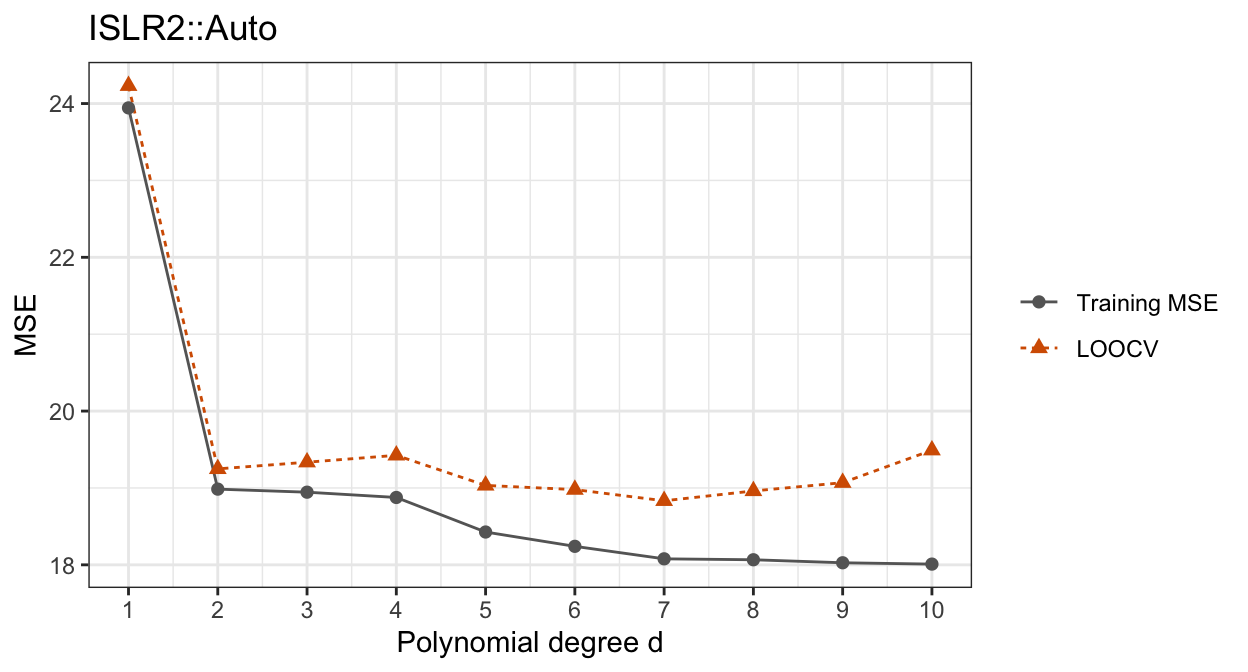

The LOOCV estimate drops from 24.23 at degree 1 to 19.25 at degree 2 and then barely moves. Its minimum, 18.83, is at degree 7, only 0.42 below the quadratic. Unlike the training MSE, it does not keep falling: at degree 10 it is 19.49, above its minimum, while the training MSE is at its lowest.

17.4 k-fold cross-validation

Code

n_folds <- 10
fold_auto <- sample(rep(seq_len(n_folds), length.out = n_auto))
fold_sizes <- table(fold_auto)

fold_roles <- c("Training", "Validation")
fold_plot <- map(seq_len(n_folds), \(l) {
  mutate(Auto, panel = paste("Fold", l, "held out"),
         role = if_else(fold_auto == l, fold_roles[2], fold_roles[1]))
}) |>
  list_rbind() |>
  mutate(panel = factor(panel, levels = paste("Fold", seq_len(n_folds), "held out")),
         role = factor(role, levels = fold_roles)) |>
  arrange(role) |>
  ggplot(aes(x = horsepower, y = mpg, color = role, shape = role, size = role)) +
  geom_point(alpha = 0.8) +
  facet_wrap(~ panel, nrow = 2) +
  scale_color_manual(values = c("grey70", "black")) +
  scale_shape_manual(values = c(16, 17)) +
  scale_size_manual(values = c(0.5, 1.3)) +
  labs(x = "Horsepower", y = "Miles per gallon", color = NULL, shape = NULL,
       size = NULL, title = "ISLR2::Auto in 10 folds") +
  theme(legend.position = "bottom")

The figure below splits the 392 cars at random into 10 groups of about equal size. Each panel marks one group as black triangles and the rest as grey circles.

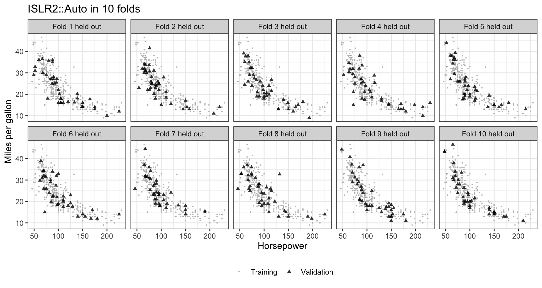
The groups hold 39 and 40 cars, and every car appears as a triangle in exactly one panel. Each group is scattered across the whole range of horsepower.

17.4.1 k-fold estimate

\(k\)-fold cross-validation divides the observations at random into \(k\) groups, or folds, \(\mathcal{F}_1, \ldots, \mathcal{F}_k\), of about equal size. For each fold \(\ell = 1, \ldots, k\) it fits the model to the other \(k - 1\) folds and computes the MSE on fold \(\ell\),

\[\text{MSE}_\ell = \frac{1}{n_\ell}\sum_{i \in \mathcal{F}_\ell}\left[y_i - \hat f^{(-\ell)}(x_i)\right]^2, \qquad \text{CV}_{(k)} = \sum_{\ell=1}^k \frac{n_\ell}{n}\,\text{MSE}_\ell,\]

where

\(k\) is the number of folds, written lowercase as in the name \(k\)-fold cross-validation; it is unrelated to \(K\), the number of neighbors in KNN (or of classes in the generative classifier lectures),
\(\mathcal{F}_\ell\) is the set of indices of the observations in fold \(\ell\) and \(n_\ell\) their number,
\(\hat f^{(-\ell)}\) is the model fit to the observations outside fold \(\ell\), and
\(\text{CV}_{(k)}\) is the average of the fold MSEs weighted by fold size, which is \(\frac{1}{k}\sum_\ell \text{MSE}_\ell\) when every fold has \(n/k\) observations, and is the average squared held-out error over all \(n\) observations.

Every observation is held out exactly once and used for fitting \(k - 1\) times. LOOCV is the special case \(k = n\), with one observation per fold.

kfold_mse <- function(d, fold, data = Auto) {
  sq_error <- numeric(nrow(data))
  for (l in unique(fold)) {
    held_out <- fold == l
    fit <- fit_degree(d, data[!held_out, ])
    sq_error[held_out] <- (data$mpg[held_out] - predict(fit, data[held_out, ]))^2
  }
  mean(sq_error)
}
kfold_10 <- map_dbl(degrees, kfold_mse, fold = fold_auto)

With the folds in the figure, the 10-fold estimate is 24.29 at degree 1 and 19.28 at degree 2, and is smallest, 19.19, at degree 7.

17.4.2 Partition variability

Code

n_partitions <- n_splits
partition_k <- c(5, 10)
kfold_curves <- expand_grid(k = partition_k, partition = seq_len(n_partitions)) |>
  mutate(fold = map(k, \(k) sample(rep(seq_len(k), length.out = n_auto))),
         mse = map(fold, \(f) map_dbl(degrees, kfold_mse, fold = f)),
         degree = list(degrees)) |>
  select(-fold) |>
  unnest(c(degree, mse))

method_labels <- c("Validation set", "5-fold", "10-fold")
resample_curves <- bind_rows(
  transmute(val_curves, method = method_labels[1], rep = split, degree, mse),
  transmute(kfold_curves, method = paste0(k, "-fold"), rep = partition, degree, mse)) |>
  mutate(method = factor(method, levels = method_labels))
resample_summary <- resample_curves |>
  group_by(method) |>
  summarize(sd_d2 = sd(mse[degree == 2]), .groups = "drop")
summary_of <- function(m, col) resample_summary[[col]][resample_summary$method == m]
chosen_by <- resample_curves |>
  group_by(method, rep) |>
  slice_min(mse, n = 1, with_ties = FALSE) |>
  ungroup()
chosen_degrees <- function(m) sort(unique(chosen_by$degree[chosen_by$method == m]))

loocv_line <- tibble(degree = degrees, mse = loocv_fast)
resample_plot <- function(m) {
  ggplot(filter(resample_curves, method == m), aes(x = degree, y = mse)) +
    geom_line(aes(group = rep), color = "grey65", linewidth = 0.3) +
    geom_line(data = loocv_line, color = "black", linetype = "dashed",
              linewidth = 1) +
    degree_axis +
    labs(x = "Polynomial degree d", y = "Estimated test MSE",
         title = paste0(m, ", ", n_partitions,
                        " random partitions; LOOCV dashed"))
}
resample_plots <- map(method_labels, resample_plot)

The 10-fold estimate above comes from one random partition of the cars. To see whether it changes from one partition to another, and by how much, the tabs below repeat the validation set curves of 100 random splits and add the curves of 100 random partitions into 5 folds and into 10 folds, each over the LOOCV curve (black, dashed), on the same axes.

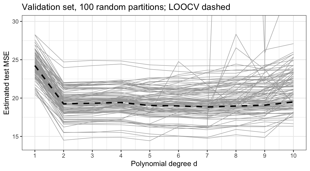
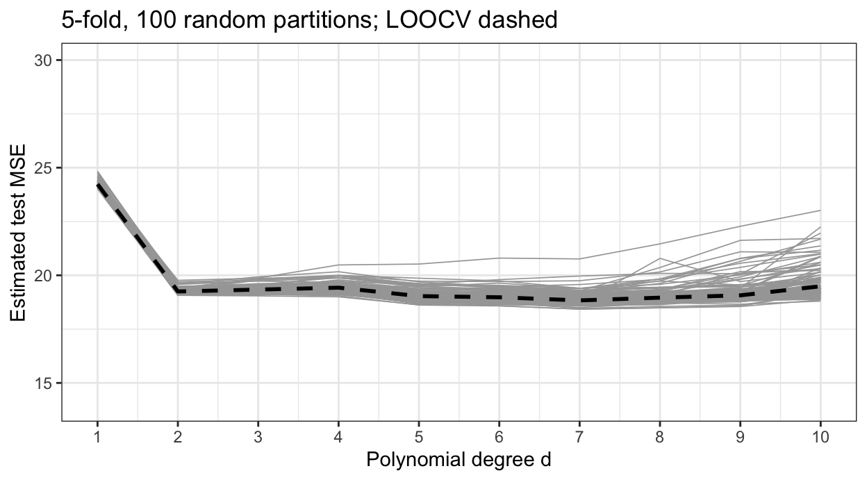
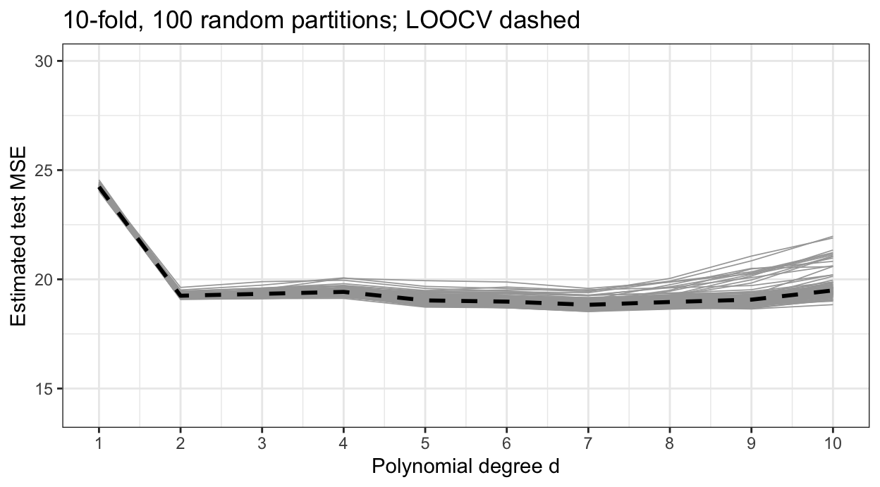
The band of curves narrows from tab to tab. At degree 2 the standard deviation of the estimate across random partitions is 1.70 for the validation set, 0.136 for 5-fold, and 0.093 for 10-fold cross-validation. The 5-fold and 10-fold curves hug the LOOCV curve, while the validation set curves scatter widely on both sides of it: every observation is held out once and the held-out errors are averaged over all \(n\) of them, so the estimate depends far less on which observations share a fold. The degree with the smallest estimate is still not fixed: across partitions 10-fold cross-validation chooses degree 2, 6, and 7, because the curves are nearly flat from degree 2 on.

17.4.3 Fold count

Any \(k\) from 2 to \(n\) gives a cross-validation estimate, and the choice affects its bias, its variance, and its computation.

Code

n_sample <- 50
n_sims <- 2000
k_values <- c(2, 5, 10, n_sample)
k_labels <- c("2-fold", "5-fold", "10-fold", paste0("LOOCV (k = ", n_sample, ")"))
k_sims <- map(seq_len(n_sims), \(r) {
  id <- sample(n_auto, n_sample)
  cars <- Auto[id, ]
  others <- Auto[-id, ]
  test_mse <- mean((others$mpg - predict(fit_degree(2, cars), others))^2)
  cv <- map_dbl(k_values, \(k) {
    if (k == n_sample) return(loocv_shortcut(2, cars))
    kfold_mse(2, sample(rep(seq_len(k), length.out = n_sample)), cars)
  })
  tibble(sim = r, method = k_labels, estimate = cv, test_mse = test_mse)
}) |>
  list_rbind() |>
  mutate(method = factor(method, levels = k_labels))
k_summary <- k_sims |>
  group_by(method) |>
  summarize(mean_estimate = mean(estimate), sd_estimate = sd(estimate),
            bias = mean(estimate - test_mse),
            se_bias = sd(estimate - test_mse) / sqrt(n()), .groups = "drop")
mean_test_mse <- mean(k_sims$test_mse[k_sims$method == k_labels[1]])
k_of <- function(m, col) k_summary[[col]][k_summary$method == m]

# A few 2-fold estimates are extreme: a quadratic fit to half of a small
# sample can extrapolate badly to a held-out car.
two_fold <- k_sims$estimate[k_sims$method == k_labels[1]]
extreme <- two_fold > 5 * mean_test_mse
n_extreme <- sum(extreme)
max_extreme <- max(two_fold)
sd_two_fold_trimmed <- sd(two_fold[!extreme])

k_plot <- ggplot(k_sims, aes(x = method, y = estimate)) +
  geom_violin(fill = "grey90", scale = "width", quantiles = c(0.25, 0.5, 0.75),
              quantile.linetype = "solid") +
  stat_summary(fun = mean, geom = "point", shape = 23, size = 3,
               fill = "#E69F00") +
  geom_hline(yintercept = mean_test_mse, linetype = "dashed") +
  coord_cartesian(ylim = quantile(k_sims$estimate, c(0.005, 0.995))) +
  labs(x = NULL, y = "Cross-validation estimate of test MSE",
       title = paste0(format(n_sims, big.mark = ","), " samples of ", n_sample,
                      " cars; quadratic fit"),
       caption = paste("Lines = quartiles and median, diamond = mean, dashed line = mean test MSE.",
                       "Vertical axis clipped to the middle 99% of the estimates."))

To see how \(k\) affects the bias and variance of the estimate, the 392 cars were treated as a population. Each of 2,000 times, a sample of 50 cars was drawn without replacement and a quadratic was fit to it; the actual test MSE of that fit is its average squared error on the 342 cars not drawn. The figure compares the cross-validation estimates from the same 50 cars, with \(k\) equal to 2, 5, 10, and 50 (LOOCV), against it. Each violin shows the distribution of one method’s estimates, with lines at its first quartile, median, and third quartile and a diamond at its mean; the dashed line is the mean test MSE.

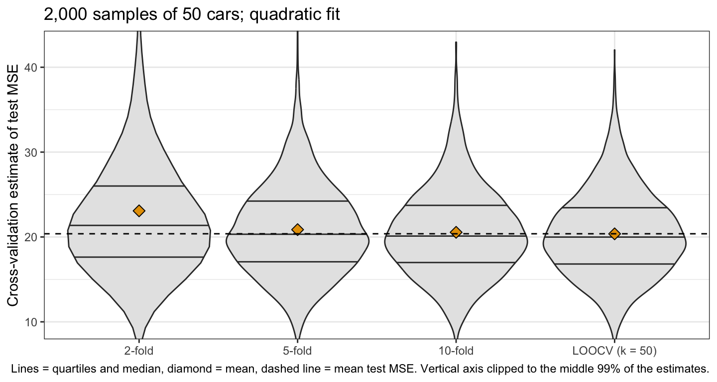
The average actual test MSE of the fits is 20.38. The estimates average 23.08 for 2-fold, 20.86 for 5-fold, 20.55 for 10-fold, and 20.37 for LOOCV. 2-fold cross-validation, fitting to 25 cars, overestimates by 2.70, with a simulation standard error of 0.52; by \(k = 5\) the overestimate is small, 0.49, with a simulation standard error of 0.14. The standard deviations of the estimates are 23.06, 5.35, 5.15, and 5.01, so 10-fold and LOOCV vary about equally. The 2-fold standard deviation is dominated by 3 of the 2,000 samples, whose estimates exceed five times the mean test MSE (the largest is 984.29), where a quadratic fit to 25 cars extrapolates badly to a held-out car; without them it is 7.61. The figure’s vertical axis is clipped, so those estimates are not shown.

Three considerations explain these results and trade off in choosing \(k\).

Computation. \(k\)-fold cross-validation needs \(k\) fits per model, LOOCV \(n\). For least squares the shortcut makes LOOCV cost one fit; for most other methods it is \(n\) fits, and \(k = 5\) or \(10\) is a large saving.
Bias. Each fit uses \(n(k-1)/k\) observations: for all 392 cars, 196 with \(k = 2\), about 314 with \(k = 5\), about 353 with \(k = 10\), and 391 with LOOCV. By the learning curve above, a model fit to fewer observations has larger test error, so \(\text{CV}_{(k)}\) overestimates the test error of the model fit to all \(n\), by more as \(k\) shrinks. LOOCV is nearly unbiased.
Variance. \(\text{CV}_{(k)}\) is an average of \(k\) fold MSEs. If each has variance \(\tau^2\) and each pair has correlation \(\rho\),

\[Var\left[\frac{1}{k}\sum_{\ell=1}^k\text{MSE}_\ell\right] = \frac{1}{k^2}\sum_{\ell=1}^k\sum_{\ell'=1}^k Cov\left[\text{MSE}_\ell, \text{MSE}_{\ell'}\right] = \tau^2\left(\rho + \frac{1-\rho}{k}\right),\]

where \(\ell'\) is a second fold index. Averaging more folds shrinks the \((1-\rho)/k\) term but not \(\rho\tau^2\). In LOOCV any two fits share \(n - 2\) of their \(n - 1\) observations, so their held-out errors are strongly correlated and averaging \(n\) of them reduces the variance less than the number \(n\) suggests; with larger \(k\) each fold MSE is also computed from fewer observations, raising \(\tau^2\). Which effect dominates depends on the method and the data.

The standard deviations in the simulation combine two sources: which 50 cars were drawn, shared by all four estimates, and, for \(k\)-fold, the random partition. The partition alone is the cleaner comparison. With all 392 cars held fixed, the degree-2 estimate varied across random partitions with standard deviation 0.136 for 5-fold and 0.093 for 10-fold cross-validation, and LOOCV, with no partition, does not vary at all.

For a quadratic fit to 50 cars, 5-fold and 10-fold cross-validation had small bias and variance close to LOOCV’s, and for a method without the least squares shortcut they need 5 or 10 fits rather than \(n\). That combination is why \(k = 5\) or \(10\) is the usual choice.

17.5 Classification

17.5.1 Credit card default data

Code

# The QDA lecture's split, recreated with its seed; the generator's state is
# restored afterward so this lecture's later draws are unaffected.
rng_state <- .Random.seed
set.seed(20261001)
train_id <- sample(nrow(Default), nrow(Default) / 2)
assign(".Random.seed", rng_state, envir = globalenv())
train <- Default[train_id, ]
test  <- Default[-train_id, ]

# The QDA lecture's rule of thumb: the smallest odd integer above sqrt(n).
odd_above_sqrt <- function(n) {
  k <- floor(sqrt(n))
  if (k %% 2 == 0) k + 1 else k + 2
}
K_rule <- odd_above_sqrt(nrow(train))

dollar_labels <- function(v) {
  ifelse(is.na(v), NA,
         paste0("$", format(v, big.mark = ",", scientific = FALSE, trim = TRUE)))
}
default_plot <- ggplot(arrange(train, default),
                       aes(x = balance, y = income, color = default,
                           shape = default)) +
  geom_point(alpha = 0.4, size = 0.9) +
  scale_color_manual(values = class_colors) +
  scale_shape_manual(values = c(No = 16, Yes = 17)) +
  scale_x_continuous(labels = dollar_labels) +
  scale_y_continuous(labels = dollar_labels) +
  guides(color = guide_legend(override.aes = list(alpha = 1, size = 2))) +
  labs(x = "Credit card balance ($)", y = "Income ($)", color = "Default",
       shape = "Default", title = "ISLR2::Default, training half")

The QDA and naive Bayes lecture classified ISLR2::Default credit card customers as defaulters or not from balance and income, fitting every classifier to a random half of the 10,000 customers and evaluating it on the other half. Its KNN classifier used \(K = 71\) neighbors, the smallest odd integer above \(\sqrt{n}\) for the training half, a rule of thumb. The figure below plots the same training half, recreated with the same seed.

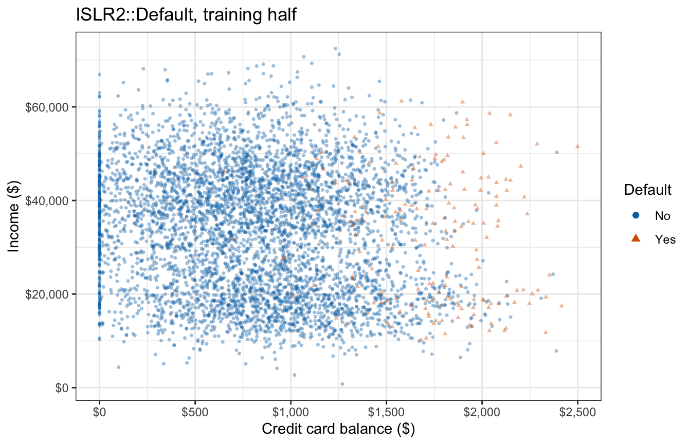
The training half holds 5,000 customers, of whom 176 (3.52%) defaulted. Defaulters sit at high balances at every income, mixed among non-defaulters with similar balances.

17.5.2 Cross-validation error rate

Cross-validation for a classifier replaces the squared error with a classification loss. With the misclassification indicator,

\[\text{Err}_\ell = \frac{1}{n_\ell}\sum_{i \in \mathcal{F}_\ell}\mathrm{I}\left(y_i \ne \hat y_i^{(-\ell)}\right), \qquad \text{CV}_{(k)} = \sum_{\ell=1}^k\frac{n_\ell}{n}\,\text{Err}_\ell,\]

where

\(\hat y_i^{(-\ell)}\) is the class predicted for observation \(i\) by the classifier fit to the observations outside fold \(\ell\), and
\(\text{Err}_\ell\) is the test error rate of that classifier on fold \(\ell\).

Any loss can take the place of the indicator. Log loss, from the classification lecture, scores the predicted probabilities rather than the classes: with \(y_i\) coded \(1\) for the positive class and \(0\) otherwise, it replaces \(\mathrm{I}\left(y_i \ne \hat y_i^{(-\ell)}\right)\) with \(-\left\{y_i\log\hat p^{(-\ell)}(x_i) + (1 - y_i)\log\left[1 - \hat p^{(-\ell)}(x_i)\right]\right\}\), where \(\hat p^{(-\ell)}(x_i)\) is the predicted probability of the positive class. A KNN vote share of exactly \(0\) or \(1\) on a misclassified observation makes it infinite, so log loss suits classifiers whose probabilities stay away from \(0\) and \(1\), such as logistic regression.

For KNN, the classifier fit to the training folds includes the standardization of the features: their means and standard deviations are computed from the training folds, as they were computed from the training half in the QDA lecture.

features <- c("balance", "income")
knn_classify <- function(fit_data, new_data, K) {
  center <- colMeans(fit_data[features])
  spread <- map_dbl(fit_data[features], sd)
  class::knn(scale(fit_data[features], center, spread),
             scale(new_data[features], center, spread),
             fit_data$default, k = K)
}
knn_cv_error <- function(K, fold, data = train) {
  wrong <- logical(nrow(data))
  for (l in unique(fold)) {
    held_out <- fold == l
    predicted <- knn_classify(data[!held_out, ], data[held_out, ], K)
    wrong[held_out] <- predicted != data$default[held_out]
  }
  mean(wrong)
}

17.5.3 Neighbor count

Code

fold_default <- sample(rep(seq_len(n_folds), length.out = nrow(train)))
K_grid <- seq(1, 201, by = 2)
knn_errors <- tibble(K = K_grid) |>
  mutate(Training = map_dbl(K, \(K) mean(knn_classify(train, train, K) != train$default)),
         `10-fold CV` = map_dbl(K, knn_cv_error, fold = fold_default),
         `Test half` = map_dbl(K, \(K) mean(knn_classify(train, test, K) != test$default)))
K_cv <- knn_errors$K[which.min(knn_errors$`10-fold CV`)]
K_test <- knn_errors$K[which.min(knn_errors$`Test half`)]
share_test_below <- mean(knn_errors$`Test half` < knn_errors$`10-fold CV`)
knn_of <- function(K_value, col) knn_errors[[col]][knn_errors$K == K_value]
test_below_cv_min <- knn_of(K_cv, "Test half") < min(knn_errors$`10-fold CV`)

knn_long <- knn_errors |>
  pivot_longer(-K, names_to = "error", values_to = "rate") |>
  mutate(error = factor(error, levels = c("Training", "10-fold CV", "Test half")))
knn_plot <- ggplot(knn_long, aes(x = 1 / K, y = rate, color = error,
                                 linetype = error, shape = error)) +
  geom_vline(xintercept = 1 / c(K_cv, K_rule), color = "grey70") +
  geom_line() +
  geom_point(data = filter(knn_long, K %in% c(1, 3, 5, 11, 21, 51, 101, 201)),
             size = 2) +
  annotate("text", x = 1 / c(K_cv, K_rule), y = max(knn_long$rate), hjust = -0.1,
           label = c(paste("K =", K_cv, "(CV)"), paste("K =", K_rule, "(rule)")),
           size = 3) +
  scale_x_log10(breaks = 1 / c(1, 3, 10, 30, 100, 200),
                labels = c("1", "1/3", "1/10", "1/30", "1/100", "1/200")) +
  scale_y_continuous(labels = \(v) paste0(100 * v, "%")) +
  scale_color_manual(values = c("grey40", "#D55E00", "#0072B2")) +
  labs(x = "Flexibility 1/K (log scale)", y = "Error rate", color = NULL,
       linetype = NULL, shape = NULL, title = "KNN on ISLR2::Default")

The training half was divided into 10 folds, and the 10-fold cross-validation error rate was computed for every odd \(K\) from 1 to 201. The figure plots it against \(1/K\), the flexibility, with the training error rate and the error rate on the test half for comparison.

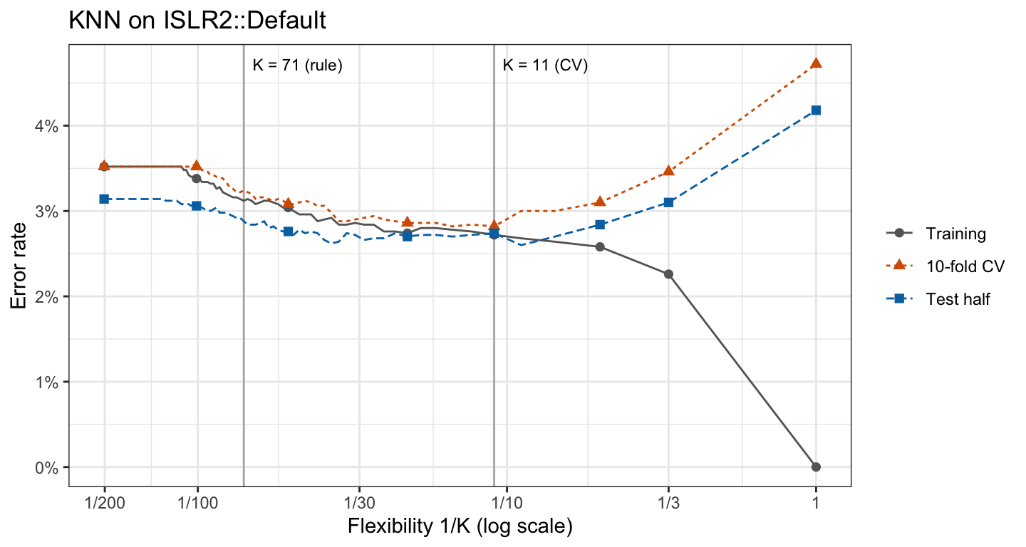
The training error rate falls to 0.00% at \(K = 1\), where every training customer is its own nearest neighbor. The cross-validation error rate is U-shaped instead: 4.72% at \(K = 1\), a minimum of 2.82% at \(K = 11\), and 3.52% at \(K = 201\), where KNN classifies every customer as a non-defaulter and its error rate equals the proportion of defaulters. The rule of thumb’s \(K = 71\) has a cross-validation error rate of 3.24%.

The test half, which the cross-validation never touched, gives the same shape: its error rate is 2.74% at \(K = 11\) and 2.88% at \(K = 71\), and is smallest, 2.60%, at \(K = 9\). The test curve lies below the cross-validation curve at every value of \(K\), in part because defaulters are rarer in the test half, 3.14% against 3.52%, which also sets the level of each curve at large \(K\).

17.6 Data-dependent steps

The data sets in this section have thousands of features and only dozens of observations, and none of the features carries any information about the response. They are simulated rather than real because the point concerns the data-generating process: with no information in the features, the true test error rate of any classifier is known, so a cross-validation estimate can be checked against it.

17.6.1 Noise feature screening

Code

n_noise <- 50
p_noise <- 5000
q_keep <- 20
K_noise <- 5
# Two classes of equal size and no information in the features.
true_error <- 1 / 2
simulate_noise <- function() {
  list(X = matrix(rnorm(n_noise * p_noise), n_noise, p_noise),
       y = factor(rep(c("A", "B"), each = n_noise / 2)))
}
screen <- function(X, y, q) {
  order(abs(cor(X, as.numeric(y))), decreasing = TRUE)[seq_len(q)]
}

noise_example <- simulate_noise()
top_two <- screen(noise_example$X, noise_example$y, 2)
top_cor <- abs(cor(noise_example$X[, top_two], as.numeric(noise_example$y)))
# Which class sits higher (second feature) and further right (first feature).
class_means <- sapply(top_two, \(j) tapply(noise_example$X[, j], noise_example$y, mean))
upper_class <- rownames(class_means)[which.max(class_means[, 2])]
right_class <- rownames(class_means)[which.max(class_means[, 1])]
other_class <- function(cl) setdiff(levels(noise_example$y), cl)
noise_plot <- tibble(first = noise_example$X[, top_two[1]],
                     second = noise_example$X[, top_two[2]],
                     class = noise_example$y) |>
  ggplot(aes(x = first, y = second, color = class, shape = class)) +
  geom_point(size = 2.2) +
  scale_color_manual(values = c(A = "#0072B2", B = "#D55E00")) +
  labs(x = paste("Feature", top_two[1]), y = paste("Feature", top_two[2]),
       color = "Class", shape = "Class",
       title = paste("The two of", format(p_noise, big.mark = ","),
                     "noise features most correlated with the class"))

Each simulated data set has \(n = 50\) observations in two classes of 25 and \(p = 5{,}000\) features, all independent standard normal draws unrelated to the class, so the true test error rate of any classifier is 50%. A common first step with so many features is screening: keep the 20 features most correlated with the response, then fit a classifier to those. The figure plots the two features of one data set with the largest absolute correlation with the class.

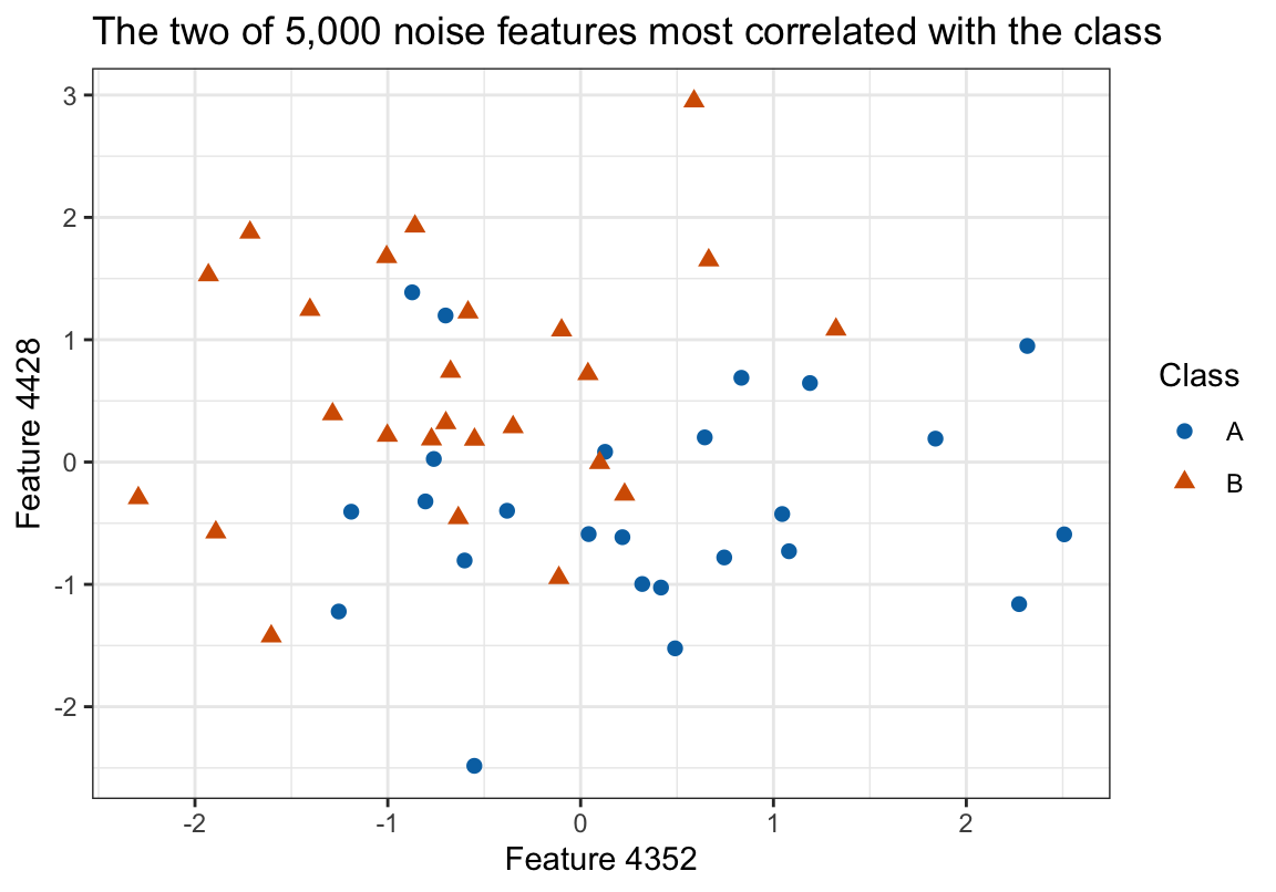
The classes look partly separated: class B tends to sit higher than class A, and class A further right than class B. The absolute correlations of these two features with the class are 0.46 and 0.46. Among 5,000 features unrelated to the class, some are correlated with it in a sample of 50 by chance, and screening finds exactly those.

17.6.2 Within-fold screening

The function below estimates the error rate of “screen the 20 most correlated features, then classify by KNN with \(K = 5\)” by 10-fold cross-validation, in one of two ways. With inside = FALSE it screens once, on all \(n\) observations, and cross-validates only the KNN step. With inside = TRUE it screens again within each fold, using only the training folds.

screen_cv_error <- function(X, y, inside,
                            fold = sample(rep(seq_len(n_folds), length.out = nrow(X)))) {
  keep_all <- screen(X, y, q_keep)
  wrong <- logical(nrow(X))
  for (l in seq_len(n_folds)) {
    held_out <- fold == l
    keep <- if (inside) screen(X[!held_out, ], y[!held_out], q_keep) else keep_all
    predicted <- class::knn(X[!held_out, keep], X[held_out, keep, drop = FALSE],
                            y[!held_out], k = K_noise)
    wrong[held_out] <- predicted != y[held_out]
  }
  mean(wrong)
}

Code

n_noise_sims <- 200
screen_labels <- c("Screen once, then cross-validate",
                   "Screen inside each fold")
screen_sims <- map(seq_len(n_noise_sims), \(r) {
  d <- simulate_noise()
  tibble(approach = screen_labels,
         error = c(screen_cv_error(d$X, d$y, inside = FALSE),
                   screen_cv_error(d$X, d$y, inside = TRUE)))
}) |>
  list_rbind() |>
  mutate(approach = factor(approach, levels = screen_labels))
screen_mean <- function(a) mean(screen_sims$error[screen_sims$approach == a])

# Screening inside each fold on further data sets, three ways: folds drawn as
# above; stratified folds, each holding equally many of each class; and class
# labels drawn independently rather than fixed at n / 2 per class.
n_check_sims <- 1000
stratified_fold <- function(y) {
  fold <- integer(length(y))
  for (cl in levels(y)) {
    fold[y == cl] <- sample(rep(seq_len(n_folds), length.out = sum(y == cl)))
  }
  fold
}
check_labels <- c("random", "stratified", "independent")
inside_checks <- map(seq_len(n_check_sims), \(r) {
  d <- simulate_noise()
  y_independent <- factor(sample(levels(d$y), n_noise, replace = TRUE),
                          levels = levels(d$y))
  tibble(folds = check_labels,
         error = c(screen_cv_error(d$X, d$y, inside = TRUE),
                   screen_cv_error(d$X, d$y, inside = TRUE,
                                   fold = stratified_fold(d$y)),
                   screen_cv_error(d$X, y_independent, inside = TRUE)))
}) |>
  list_rbind() |>
  group_by(folds) |>
  summarize(mean = mean(error), se = sd(error) / sqrt(n()), .groups = "drop")
check_of <- function(f, col = "mean") inside_checks[[col]][inside_checks$folds == f]

screen_plot <- ggplot(screen_sims, aes(x = error)) +
  geom_histogram(binwidth = 0.04, boundary = 0, fill = "grey60", color = "white") +
  geom_vline(xintercept = true_error, linetype = "dashed") +
  facet_wrap(~ approach, ncol = 1) +
  scale_x_continuous(labels = \(v) paste0(100 * v, "%"), limits = c(0, 1)) +
  labs(x = "10-fold cross-validation error rate", y = "Simulated data sets",
       title = paste0(n_noise_sims, " simulated data sets; true error rate ",
                      pct(true_error, 0), " (dashed)"))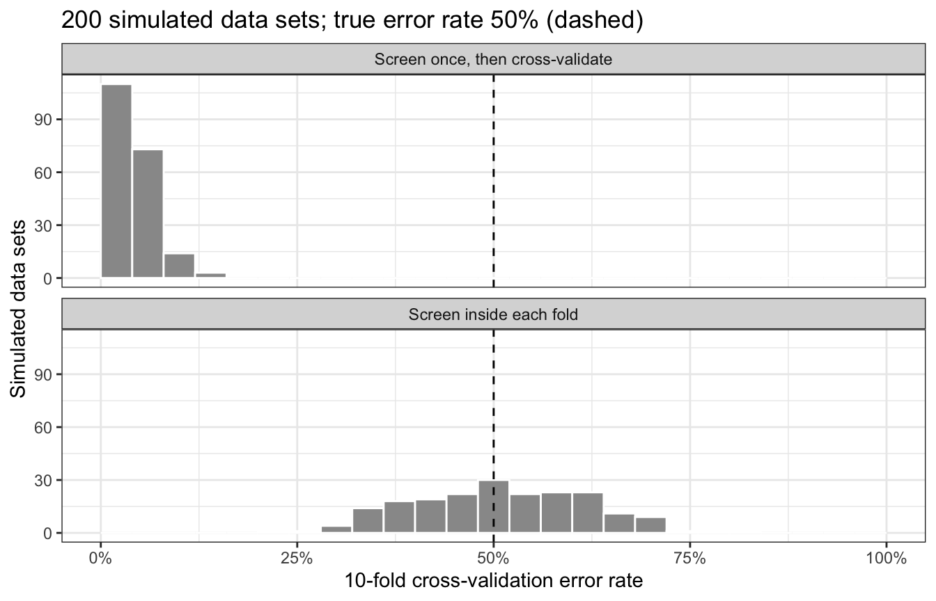

Across 200 simulated data sets, screening once and then cross-validating gives an average estimated error rate of 5.1%, against a true error rate of 50%. Screening inside each fold gives 51.8%. The first approach selected the features using the responses of the very observations it later held out, so those observations were not new to the classifier.

Screening is part of the fit. So is every other step that uses the data to build a classifier or a regression, and a cross-validation estimate is honest only if all of those steps are repeated, inside every fold, using only the training folds.

The second estimate sits slightly above 50%. To see why, screening inside each fold was cross-validated on 1,000 further simulated data sets in three ways. With folds drawn at random as above, the average estimated error rate is 51.8%. With stratified folds, each holding equally many observations of each class, it is 50.1%. With each class label drawn independently, A and B equally likely, so that the class counts vary from one data set to the next, it is 49.9%. Each of these averages has a simulation standard error of at most 0.33 percentage points.

Only the first combines fixed class counts with folds that ignore the class. Each data set has exactly 25 observations per class, so a held-out fold with more of one class leaves the training folds with fewer of it. A classifier with no information leans toward the class that is more common in its training folds, which is the less common class in the held-out fold. Stratified folds remove the imbalance between held-out and training folds, and independent labels remove the fixed counts that tie them together, and both estimates are within simulation error of 50%.

17.6.3 Standardization and tuning

Standardization follows the same rule as screening; tuning does not.

Standardization. knn_classify() computes the feature means and standard deviations from the training folds and applies them to the held-out fold. Standardizing the whole data set first lets the held-out observations influence the scale, the same kind of leak as screening.
Tuning. Choosing \(K\) by cross-validation is itself a data-dependent step. The smallest of 101 cross-validation error rates, 2.82%, is the minimum of noisy estimates, so over repeated data sets it tends to fall below the test error rate of the classifier it chooses. An honest estimate of the error of “choose \(K\) by 10-fold cross-validation, then fit” needs data not used in the choosing: here the test half, where \(K = 11\) has error rate 2.74%. On this one split that is below the cross-validation minimum, the opposite of the tendency, because the test curve lies below the cross-validation curve.

Beyond this course

One-standard-error rule. When the cross-validation curve is nearly flat near its minimum, as for the polynomial degree of the cars, choose the simplest model whose estimate is within one standard error of the minimum, the standard error computed from the \(k\) fold MSEs.
Repeated and stratified \(k\)-fold. Averaging \(k\)-fold estimates over several random partitions reduces their dependence on the partition; stratifying the folds keeps the class proportions the same in every fold, which matters when one class is rare, as defaulters are.
Nested cross-validation. An outer cross-validation loop around the whole procedure “choose the tuning parameter by inner cross-validation, then fit” estimates the test error of that procedure without a separate test set.

17.7 Conclusion

Training error falls as flexibility increases, so it cannot choose a model’s flexibility. Resampling methods estimate test error by fitting to part of the data and measuring error on the part held out.

The validation set approach holds out one random part. Its estimate varies with the split, and because each model is fit to only part of the data it tends to overestimate the test error of the model fit to all \(n\). Leave-one-out cross-validation holds out each observation in turn and averages the \(n\) squared held-out errors. It involves no random split and is nearly unbiased. For least squares it needs a single fit, since the held-out error of observation \(i\) is its residual divided by \(1 - h_i\).

\(k\)-fold cross-validation divides the data into \(k\) folds, fits \(k\) times, and averages the held-out errors. Choosing \(k\) trades bias, variance, and computation. Smaller \(k\) means smaller training sets and so more upward bias; larger \(k\) averages more, but more strongly correlated, fold errors, so its variance falls more slowly than the number of folds suggests; and each additional fold is another fit. \(k = 5\) or \(10\) is the usual choice because each fit uses 80% or 90% of the data, which keeps the bias modest, while a method without the least squares shortcut needs only 5 or 10 fits rather than \(n\). For classification the squared error becomes the misclassification indicator or another loss such as log loss, and the cross-validation curve chooses a flexibility setting, such as the number of neighbors in KNN, as it chooses a polynomial degree.

A cross-validation estimate is honest only when every data-dependent step, including feature screening and standardization, is repeated inside each fold using only the training folds. Selecting features on all the data first lets the held-out observations shape the fit, and the estimate becomes optimistic. Choosing a tuning parameter by the smallest cross-validation estimate is itself a data-dependent choice, so that minimum tends to be optimistic as well.

The next lecture puts cross-validation into practice: choosing among models and tuning parameters on real data, and the issues that choosing raises.