15 Quadratic Discriminant Analysis and Naive Bayes

Learning objectives

After this lecture you should be able to

derive the QDA discriminant function $\delta_k(x)$ from Gaussian class-conditional densities with class-specific covariance matrices $\Sigma_k$, and show that the resulting decision boundary is quadratic in $x$, with up to two boundary points when $p = 1$,
count the mean and covariance parameters that LDA, QDA, and Gaussian naive Bayes estimate, and use the counts to explain through the bias-variance tradeoff when each should have the lowest test error rate,
write the naive Bayes model, with the features conditionally independent given the class, in $\stackrel{ind}{\sim}$ notation over observations and features, write $f_k(x)$ as a product of one-feature densities of possibly different types, show that the log posterior odds are a sum of one-feature terms, and identify Gaussian naive Bayes as LDA or QDA with a diagonal covariance matrix,
define the KNN estimate of $p_k(x_0)$ as the proportion of the $K$ nearest neighbors, on standardized features, in class $k$, and the KNN classifier as the class with the largest estimate,
compare logistic regression, LDA, QDA, naive Bayes, and KNN by the functional form of their log posterior odds, including logistic regression with squared and cross-product features, their assumptions, how they estimate their parameters, and how they are affected by $n$ and $p$, and evaluate which should perform best in a described setting, and
fit QDA with MASS::qda(), naive Bayes with e1071::naiveBayes(), and KNN with class::knn(), interpret their output, and compare classifiers by test error rate, sensitivity, specificity, and AUC on a held-out test set.

15.1 Generative classifiers

15.1.1 Credit card default data

Question. Do quadratic discriminant analysis (QDA) and naive Bayes, which change LDA’s model of the features in different directions, classify credit card customers more accurately than LDA and logistic regression, and how does K-nearest neighbors (KNN) compare?

These customers were analyzed in the logistic regression lectures and, with balance and income as the features, in the Linear Discriminant Analysis lecture, which modeled each class’s features by a Gaussian density with one covariance matrix shared by both classes. The Classifier Evaluation lecture then measured how well those fits classify them.

Data. ISLR2::Default is a simulated data set of 10,000 credit card customers. The response is default, with Yes the positive class. The explanatory variables are balance, the customer’s monthly credit card balance in dollars, and income, the customer’s income in dollars; the features are the explanatory variables themselves. student (Yes/No) enters only as a third, binary feature of naive Bayes, in the naive Bayes section’s mixed feature types and again in the Student strata section, where it also splits the customers.

The previous lecture’s error rates were training error rates, optimistic on average because each customer helped fit the model that classified it. Here, as in the classification lecture’s bias-variance script, the customers are first split at random into halves: every model in this lecture is fit to the training half and evaluated on the test half, whose customers it never saw.

Code

# Its own seed, so the split does not depend on anything drawn before it.
set.seed(20261001)
train_id <- sample(nrow(Default), nrow(Default) / 2)
train <- Default[train_id, ]
test  <- Default[-train_id, ]

n_defaults <- c(train = sum(train$default == "Yes"),
                test  = sum(test$default == "Yes"))

Each half holds 5,000 customers, with 176 defaulters in the training half and 157 in the test half. A different split would give somewhat different test error rates; averaging over many splits is a topic of the resampling unit.

The figure below plots income against balance for the training customers, defaulters and non-defaulters distinguished by color and shape, with each class’s approximately 95% normal-theory ellipse (solid for non-defaulters, dashed for defaulters), a contour of a Gaussian density with that class’s sample mean and covariance matrix.

Code

class_summary <- train |>
  group_by(default) |>
  summarize(sd_balance = sd(balance), sd_income = sd(income),
            cor_balance_income = cor(balance, income), .groups = "drop")
summary_of <- function(k, col) class_summary[[col]][class_summary$default == k]
student_income <- function(s) median(train$income[train$student == s])

# Defaulters are drawn last so they are not hidden under non-defaulters.
scatter_points <- list(
  geom_point(data = arrange(train, default),
             aes(x = balance, y = income, color = default, shape = default),
             alpha = 0.35, size = 0.8),
  scale_color_manual(values = class_colors),
  scale_shape_manual(values = c(16, 17)),
  scale_x_continuous(labels = dollar_labels),
  scale_y_continuous(labels = dollar_labels),
  labs(x = "Credit card balance ($)", y = "Income ($)", color = "Default",
       shape = "Default")
)
eda_scatter <- ggplot() +
  scatter_points +
  stat_ellipse(data = train, aes(x = balance, y = income, color = default,
                                 linetype = default),
               type = "norm", level = 0.95, linewidth = 0.9) +
  guides(color = guide_legend(override.aes = list(alpha = 1, size = 2))) +
  labs(linetype = "Default",
       title = "Training set, with each class's approximately 95% normal-theory ellipse")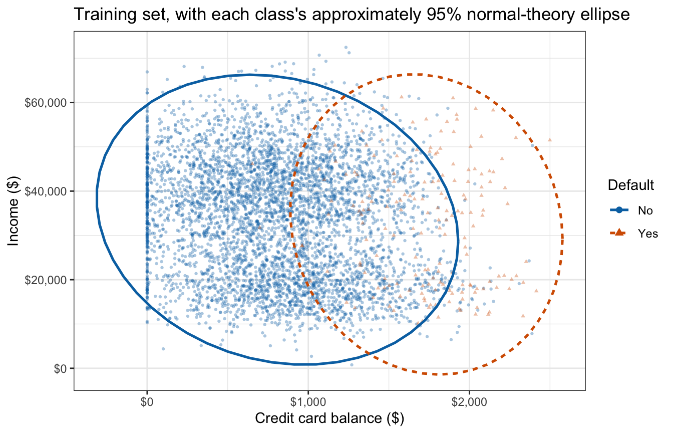

The defaulters’ ellipse is centered at higher balances and is narrower in the balance direction: the standard deviation of balance is $458 among non-defaulters and $342 among defaulters. Income is about equally spread in the two classes, with standard deviations of $13,370 and $13,731.

Within each class balance and income are weakly correlated, with $r = -0.150$ among non-defaulters and $r = -0.096$ among defaulters, so both ellipses are only slightly tilted. Among non-defaulters the points are densest in two horizontal bands, the bimodal income of the LDA lecture’s histograms. The lower band is mostly students: in the training half students’ median income is $17,980, against $40,135 for non-students. No Gaussian density has two modes.

15.1.2 Bayes’ theorem and LDA

With the response in one of $K$ classes, $k = 1, \ldots, K$, the previous lecture built a classifier from the prior probabilities $\pi_k = P(Y = k)$ and the class-conditional densities $f_k(x)$ of the features through Bayes’ theorem,

\[p_k(x) = P(Y = k \mid X = x) = \frac{\pi_k f_k(x)}{\sum_{l=1}^K \pi_l f_l(x)},\]

and assigned each observation to the class with the largest posterior probability. Every generative classifier in this course estimates $\pi_k$ by the class proportion $n_k/n$, where $n_k$ is the number of training observations in class $k$ and $n$ the number of training observations. They differ only in the model assumed for $f_k(x)$.

LDA assumed, for observations $i = 1, \ldots, n$, $Y_i \stackrel{ind}{\sim} \text{Categorical}\left(\pi_1, \ldots, \pi_K\right)$ and $X_i \mid Y_i = k \stackrel{ind}{\sim} N_p\left(\mu_k, \Sigma\right)$, with $X_i$ the random $p$-vector of features of observation $i$ and one covariance matrix $\Sigma$ shared by every class. That is what made the quadratic term in $x$ cancel and the boundary linear. It would give the two ellipses of the scatterplot the same shape, but the defaulters’ is the narrower in balance.

This lecture changes the model for $f_k(x)$ in two directions. Quadratic discriminant analysis gives each class its own covariance matrix. Naive Bayes drops the multivariate Gaussian and treats the features as independent within each class. K-nearest neighbors then drops the model for $f_k(x)$ altogether and classifies by a vote of nearby training observations.

15.2 Quadratic discriminant analysis

The figure below repeats the training scatterplot of income against balance, points colored and shaped by default status, with each class’s approximately 95% normal-theory ellipse (solid for non-defaulters, dashed for defaulters).

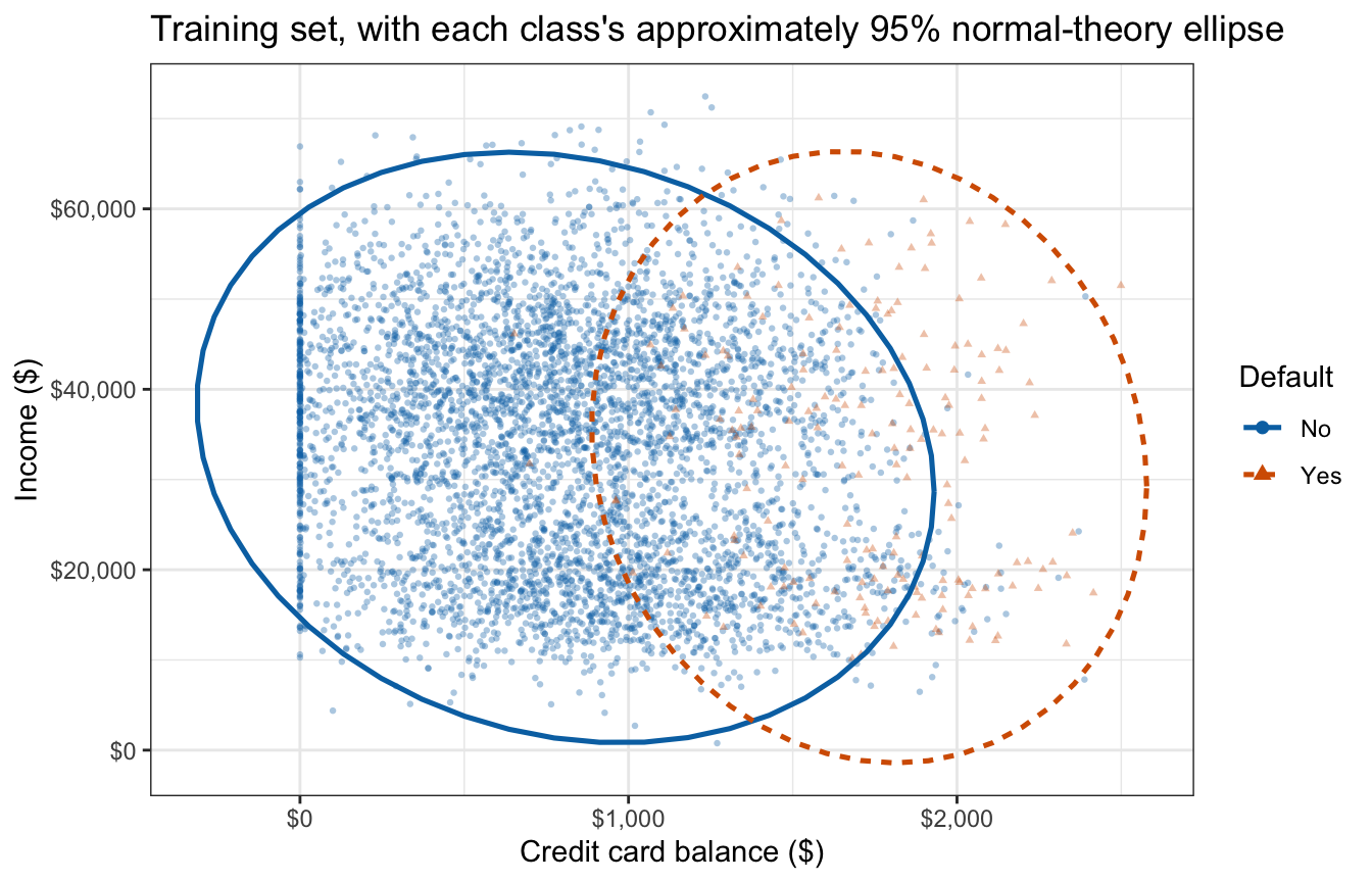
The two ellipses differ in width: the defaulters’ is narrower in balance, with standard deviation $342 against $458. One covariance matrix shared by both classes cannot describe both clouds; QDA gives each class its own.

15.2.1 Class-specific covariance matrices

Quadratic discriminant analysis (QDA) assumes the statistical model

\[Y_i \stackrel{ind}{\sim} \text{Categorical}\left(\pi_1, \ldots, \pi_K\right), \qquad X_i \mid Y_i = k \stackrel{ind}{\sim} N_p\left(\mu_k, \Sigma_k\right), \qquad i = 1, \ldots, n,\]

where

$Y_i$ is the class of observation $i$ and $X_i = (X_{i1}, \ldots, X_{ip})^\top$ its random $p$-vector of features, with observed values $y_i$ and $x_i$,
$\text{Categorical}\left(\pi_1, \ldots, \pi_K\right)$ is the distribution on the classes $\{1, \ldots, K\}$ with $P(Y_i = k) = \pi_k$,
$\stackrel{ind}{\sim}$ means independent over observations $i$, as in LDA,
$\mu_k = E[X_i \mid Y_i = k]$ is the $p$-vector of feature means in class $k$, as in LDA, and
$\Sigma_k = Cov[X_i \mid Y_i = k]$ is the $p \times p$ covariance matrix of the features in class $k$, symmetric and positive definite, and free to differ from class to class.

The class-conditional density is therefore

\[f_k(x) = \frac{1}{(2\pi)^{p/2}\left|\Sigma_k\right|^{1/2}} \exp\left[-\frac{1}{2}\left(x - \mu_k\right)^\top \Sigma_k^{-1} \left(x - \mu_k\right)\right],\]

where $\left|\Sigma_k\right|$ is the determinant of $\Sigma_k$. Each class’s contours are still ellipses centered at $\mu_k$, but now each class’s ellipses have their own size, shape, and orientation, as the two ellipses of the scatterplot do.

15.2.2 Class-specific covariance estimates

The priors and means are estimated as in LDA, $\hat\pi_k = n_k/n$ and $\hat\mu_k = \frac{1}{n_k}\sum_{i:\, y_i = k} x_i$. Each covariance matrix is estimated from its own class alone,

\[\hat\Sigma_k = \frac{1}{n_k - 1}\sum_{i:\, y_i = k}\left(x_i - \hat\mu_k\right)\left(x_i - \hat\mu_k\right)^\top,\]

where

$x_i$ is the observed $p$-vector of feature values of observation $i$, as in the LDA lecture, and
$\hat\Sigma_k$ is the class-$k$ sample covariance matrix, whose divisor $n_k - 1$ accounts for the one estimated mean.

MASS::qda() uses this divisor (maximum likelihood would use $n_k$), and $\hat\Sigma_k$, whose rank is at most $n_k - 1$, is invertible only if $n_k > p$. It takes the same formula as MASS::lda(); fitting default on balance and income in the training half:

default_qda <- MASS::qda(default ~ balance + income, data = train)
default_qda

Call:
qda(default ~ balance + income, data = train)

Prior probabilities of groups:
    No    Yes 
0.9648 0.0352 

Group means:
      balance   income
No   808.2541 33549.49
Yes 1732.5500 32482.56

Code

qda_par <- map(c(No = "No", Yes = "Yes"), \(k) {
  X <- as.matrix(train[train$default == k, c("balance", "income")])
  list(prior = mean(train$default == k), mu = colMeans(X), Sigma = cov(X))
})
# A 2 x 2 matrix as LaTeX, entries rounded with LaTeX-safe thousands commas.
matrix_tex <- function(S) {
  e <- format(round(S), big.mark = "{,}", trim = TRUE)
  sprintf("\\begin{pmatrix} %s & %s \\\\ %s & %s \\end{pmatrix}",
          e[1, 1], e[1, 2], e[2, 1], e[2, 2])
}

The output reports the prior probabilities and the class means of balance and income, the same priors and means MASS::lda() reports for these training customers; the priors differ slightly from the LDA lecture’s all-customer fit, $\hat\pi_{\text{Yes}} = 0.0333$. The covariance matrices are not printed. They are each class’s sample covariance matrix of (balance, income), in squared dollars,

\[\hat\Sigma_{\text{No}} = \begin{pmatrix} 210{,}058 & -917{,}043 \\ -917{,}043 & 178{,}743{,}544 \end{pmatrix}, \qquad \hat\Sigma_{\text{Yes}} = \begin{pmatrix} 117{,}154 & -449{,}601 \\ -449{,}601 & 188{,}550{,}929 \end{pmatrix},\]

whose square-rooted diagonals and correlations are the standard deviations and correlations quoted with the scatterplot, and whose contours are its ellipses.

15.2.3 Quadratic discriminant

As in LDA, the class with the largest posterior probability is the class with the largest $\log\left[\pi_k f_k(x)\right]$,

\[\log\left[\pi_k f_k(x)\right] = \log \pi_k - \frac{p}{2}\log(2\pi) - \frac{1}{2}\log\left|\Sigma_k\right| - \frac{1}{2}\left(x - \mu_k\right)^\top \Sigma_k^{-1}\left(x - \mu_k\right).\]

Only the term $-\frac{p}{2}\log(2\pi)$ is common to every class. Dropping it gives the quadratic discriminant function

\[\delta_k(x) = -\frac{1}{2}x^\top \Sigma_k^{-1} x + x^\top \Sigma_k^{-1}\mu_k - \frac{1}{2}\mu_k^\top \Sigma_k^{-1}\mu_k - \frac{1}{2}\log\left|\Sigma_k\right| + \log \pi_k,\]

after expanding the quadratic form as in the LDA lecture. Two terms that LDA dropped survive here:

$-\frac{1}{2}x^\top \Sigma_k^{-1} x$ is quadratic in $x$ and carries a different matrix in each class, and
$-\frac{1}{2}\log\left|\Sigma_k\right|$ penalizes a class whose density is spread over a larger volume.

When every $\Sigma_k$ equals a common $\Sigma$, both terms are the same in every class, drop out, and $\delta_k(x)$ reduces to the LDA discriminant.

With $K = 2$ classes the log posterior odds of class $2$ are

\[\log\left[\frac{p_2(x)}{1 - p_2(x)}\right] = \delta_2(x) - \delta_1(x) = \beta_0 + x^\top\left(\Sigma_2^{-1}\mu_2 - \Sigma_1^{-1}\mu_1\right) - \frac{1}{2}x^\top \left(\Sigma_2^{-1} - \Sigma_1^{-1}\right) x,\]

where

$\beta_0 = \log(\pi_2/\pi_1) - \frac{1}{2}\left(\mu_2^\top \Sigma_2^{-1}\mu_2 - \mu_1^\top \Sigma_1^{-1}\mu_1\right) - \frac{1}{2}\log\left(\left|\Sigma_2\right| / \left|\Sigma_1\right|\right)$ is the intercept, collecting the terms that do not involve $x$.

The log posterior odds are a quadratic function of the features: an intercept, $p$ linear terms $x_j$, where $x_j$ is the $j$th entry of $x$, and $p(p+1)/2$ squares $x_j^2$ and cross-products $x_j x_l$, with coefficients determined by the $\mu_k$ and $\Sigma_k$.

Code

S_no_inv  <- solve(qda_par$No$Sigma)
S_yes_inv <- solve(qda_par$Yes$Sigma)
m_no  <- qda_par$No$mu
m_yes <- qda_par$Yes$mu
A_qda <- -0.5 * (S_yes_inv - S_no_inv)
b_qda <- drop(S_yes_inv %*% m_yes - S_no_inv %*% m_no)
c_qda <- log(qda_par$Yes$prior / qda_par$No$prior) -
  0.5 * (sum(m_yes * (S_yes_inv %*% m_yes)) - sum(m_no * (S_no_inv %*% m_no))) -
  0.5 * log(det(qda_par$Yes$Sigma) / det(qda_par$No$Sigma))
balance_sq_coef <- A_qda[1, 1]

# Log posterior odds of Yes from the coefficients, checked against predict().
X_train <- as.matrix(train[c("balance", "income")])
qda_log_odds <- c_qda + drop(X_train %*% b_qda) + rowSums((X_train %*% A_qda) * X_train)
max_diff_qda <- max(abs(plogis(qda_log_odds) -
                        predict(default_qda)$posterior[, "Yes"]))

# Income in thousands of dollars, so the coefficients have readable sizes.
qda_coef_table <- tibble(
  term = c("Intercept $\\hat\\beta_0$", "$\\texttt{balance}$",
           "$\\texttt{income}$, per \\$1,000", "$\\texttt{balance}^2$",
           "$\\texttt{balance} \\times \\texttt{income}$, per \\$1,000",
           "$\\texttt{income}^2$, per (\\$1,000)$^2$"),
  value = c(c_qda, b_qda[1], 1000 * b_qda[2], A_qda[1, 1],
            2 * 1000 * A_qda[1, 2], 1e6 * A_qda[2, 2])
) |>
  mutate(value = map_chr(value, \(v) paste0("$", num_tex(v), "$"))) |>
  knitr::kable(col.names = c("Term", "Coefficient"), align = "lc")

For the credit card fit, the table gives the coefficients of QDA’s estimated log posterior odds of default, with income terms per $1,000 of income.

Term	Coefficient
Intercept $\hat\beta_0$	$-14.5$
$\texttt{balance}$	$0.0108$
$\texttt{income}$, per $1,000	$-2.73 \times 10^{-3}$
$\texttt{balance}^2$	$-1.87 \times 10^{-6}$
$\texttt{balance} \times \texttt{income}$, per $1,000	$4.44 \times 10^{-6}$
$\texttt{income}^2$, per ($1,000)$^2$	$1.85 \times 10^{-4}$

The intercept is the log posterior odds of default for a customer with no balance and no income, an extrapolation, since the lowest recorded income is $772. With squared and cross-product terms, no single coefficient gives a feature’s effect: as in the polynomial logistic regressions of the flexible logistic regression lecture, the effect of balance depends on the balance and income at which it is evaluated. Applying the logistic function to these log posterior odds reproduces predict()’s posterior probabilities to within $7 \times 10^{-15}$.

15.2.4 Quadratic decision boundary

The decision boundary, where the log posterior odds are zero, is a conic section when $p = 2$ instead of a line. With one feature, writing $\sigma_k^2$ for the class-$k$ variance, the log posterior odds are

\[\log\left[\frac{p_2(x)}{1 - p_2(x)}\right] = \frac{1}{2}\left(\frac{1}{\sigma_1^2} - \frac{1}{\sigma_2^2}\right)x^2 + \left(\frac{\mu_2}{\sigma_2^2} - \frac{\mu_1}{\sigma_1^2}\right)x + \frac{\mu_1^2}{2\sigma_1^2} - \frac{\mu_2^2}{2\sigma_2^2} + \log\frac{\sigma_1}{\sigma_2} + \log\frac{\pi_2}{\pi_1}.\]

A quadratic in $x$ has up to two roots, so the boundary is up to two points. If $\sigma_1 > \sigma_2$, the coefficient of $x^2$ is negative, the log posterior odds fall without bound in both directions, and class $1$, the class with the larger variance, is assigned in both tails. For the credit card customers class $1$ is No, whose balances have the larger standard deviation.

LDA (MASS::lda()) is refit to the same training half for contrast. The figure below draws the QDA boundary (orange, dotted) and the LDA boundary (green, solid) over the training customers, non-defaulters as grey circles and defaulters as black triangles, with balances beyond the largest training balance shaded.

Code

default_lda <- MASS::lda(default ~ balance + income, data = train)

# Each model's posterior probability of default; a model's object is looked
# up only when that model is requested, so later models can be added.
posterior_of <- function(model, d) {
  switch(model,
         "Logistic regression" = unname(predict(default_glm, newdata = d,
                                                type = "response")),
         LDA = predict(default_lda, newdata = d)$posterior[, "Yes"],
         QDA = predict(default_qda, newdata = d)$posterior[, "Yes"],
         "Naive Bayes" = predict(default_nb, newdata = d, type = "raw")[, "Yes"],
         KNN = knn_yes(d, k_default),
         "Logistic regression, squares" = unname(predict(
           squares_glm, newdata = d, type = "response")),
         "Logistic regression, squares and product" = unname(predict(
           quadratic_glm, newdata = d, type = "response")))
}
# Legend labels; the KNN label carries its number of neighbors, looked up only
# when KNN is drawn.
model_labels <- function(models) {
  map_chr(models, \(m) if (m == "KNN") paste0("KNN, K = ", k_default) else m)
}

# Balances up to `upper` at which a model's posterior crosses 0.5 at the
# training income quartiles.
income_levels <- quantile(train$income, c(0.25, 0.5, 0.75))
search_max <- 10000
crossings <- function(model, upper = search_max) {
  gap <- function(b, inc) posterior_of(model, tibble(balance = b, income = inc)) - 0.5
  map(income_levels, \(inc) {
    # Searching the generative classifiers past about $10,000 would fail:
    # e1071's naive Bayes posteriors underflow between about $15,000 and
    # $18,000 of balance, which would trip the exactly-two-crossings check
    # below.
    b <- seq(0, upper, by = 10)
    j <- which(diff(sign(gap(b, inc))) != 0)
    map_dbl(j, \(i) uniroot(gap, b[c(i, i + 1)], inc = inc)$root)
  })
}
qda_cross <- crossings("QDA")
cross_at <- function(cr, i) map_dbl(cr, i)
# The prose describes two crossings per income quartile, the second beyond
# the training data, and a negative balance^2 coefficient.
stopifnot(balance_sq_coef < 0, all(lengths(qda_cross) == 2),
          all(cross_at(qda_cross, 2) > max(train$balance)))

# Training customers under the 0.5 contour of each requested model, with
# balances beyond the largest training balance shaded. The grid reaches past
# the largest second crossing, so the second branches are always drawn.
boundary_figure <- function(models, title, second = cross_at(qda_cross, 2)) {
  grid <- expand_grid(
    balance = seq(0, max(4500, 1.15 * max(second)), length.out = 181),
    income = seq(min(Default$income), max(Default$income), length.out = 121))
  curves <- map(models, \(m) {
    mutate(grid, model = m, p_hat = posterior_of(m, grid))
  }) |>
    list_rbind() |>
    mutate(model = factor(model, levels = names(model_colors)))
  # Points are filled grey or black by default status, so that color is free
  # to identify the models' boundaries.
  ggplot(mapping = aes(x = balance, y = income)) +
    annotate("rect", xmin = max(train$balance), xmax = Inf, ymin = -Inf,
             ymax = Inf, fill = "grey92") +
    geom_point(data = arrange(train, default),
               aes(shape = default, fill = default), color = "grey40",
               stroke = 0.2, size = 1.1, alpha = 0.6) +
    geom_contour(data = curves, aes(z = p_hat, color = model, linetype = model),
                 breaks = 0.5, linewidth = 0.9) +
    scale_shape_manual(values = c(21, 24)) +
    scale_fill_manual(values = c("grey70", "black")) +
    scale_color_manual(values = model_colors, labels = model_labels) +
    scale_linetype_manual(values = model_linetypes, labels = model_labels) +
    scale_x_continuous(labels = dollar_labels) +
    scale_y_continuous(labels = dollar_labels) +
    guides(shape = guide_legend(order = 1), fill = guide_legend(order = 1),
           color = guide_legend(order = 2), linetype = guide_legend(order = 2)) +
    labs(x = "Credit card balance ($)", y = "Income ($)", shape = "Default",
         fill = "Default", color = "Model", linetype = "Model", title = title)
}
qda_boundary_plot <- boundary_figure(
  c("LDA", "QDA"), "QDA and LDA boundaries; shading beyond the largest training balance")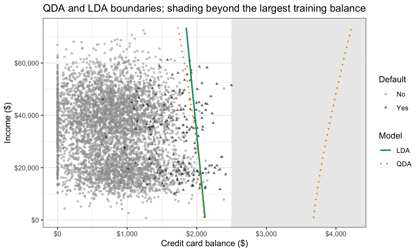

Within the training balances the QDA boundary runs close to LDA’s nearly vertical line, so income barely moves either model’s balance threshold there. Beyond them QDA’s boundary has a second branch, where its posterior probability of default falls back below $0.5$.

The second branch is easiest to see with one feature. Fitting QDA to balance alone, the first tab below plots the prior-weighted fitted densities $\hat\pi_k \hat f_k(x)$ with the class-specific standard deviations, over shaded histograms of each class’s training balances on the same scale, outlined in each class’s line type, and the second plots the two estimated discriminant functions $\hat\delta_k(x)$. Dotted lines mark the boundary points, and balances beyond the largest training balance are shaded grey.

Code

one_feature <- train |>
  group_by(default) |>
  summarize(prior = n() / nrow(train), mu = mean(balance), sd = sd(balance),
            .groups = "drop")
of_class <- function(k, col) one_feature[[col]][one_feature$default == k]

# Boundary points: roots of the one-feature log posterior odds of Yes.
m1 <- of_class("No", "mu")
s1 <- of_class("No", "sd")
m2 <- of_class("Yes", "mu")
s2 <- of_class("Yes", "sd")
log_prior_odds <- log(of_class("Yes", "prior") / of_class("No", "prior"))
roots_qda_1 <- sort(Re(polyroot(c(
  m1^2 / (2 * s1^2) - m2^2 / (2 * s2^2) + log(s1 / s2) + log_prior_odds,
  m2 / s2^2 - m1 / s1^2,
  (1 / s1^2 - 1 / s2^2) / 2))))

balance_grid_1 <- tibble(balance = seq(0, max(4500, 1.15 * roots_qda_1[2]),
                                        length.out = 600))
one_feature_curves <- one_feature |>
  cross_join(balance_grid_1) |>
  mutate(weighted = prior * dnorm(balance, mu, sd),
         delta = log(prior) - log(sd) - (balance - mu)^2 / (2 * sd^2))
one_feature_plot <- function(y, y_label, title) {
  ggplot(one_feature_curves,
         aes(x = balance, y = .data[[y]], color = default, linetype = default)) +
    annotate("rect", xmin = max(train$balance), xmax = Inf, ymin = -Inf,
             ymax = Inf, fill = "grey92") +
    geom_line(linewidth = 0.9) +
    geom_vline(xintercept = roots_qda_1, linetype = "dotted") +
    scale_color_manual(values = class_colors) +
    scale_x_continuous(labels = dollar_labels) +
    labs(x = "Credit card balance ($)", y = y_label, color = "Default",
         linetype = "Default", title = title)
}
# Histograms of training balances on the same scale as pi_k f_k: a bar's
# count divided by n times the bin width.
bin_width_1 <- 100
qda_weighted_1 <- one_feature_plot(
  "weighted", expression(hat(pi)[k] * hat(f)[k](x)),
  expression(paste("QDA prior-weighted densities, class-specific ", hat(sigma)[k]))) +
  geom_histogram(data = train,
                 aes(x = balance, y = after_stat(count) / (nrow(train) * bin_width_1),
                     fill = default, color = default, linetype = default),
                 binwidth = bin_width_1, boundary = 0, position = "identity",
                 alpha = 0.3, linewidth = 0.3, inherit.aes = FALSE) +
  scale_fill_manual(values = class_colors) +
  labs(fill = "Default")
# Vertical range from the curves' maximum down past the second crossing.
delta_at <- function(b) {
  log(of_class("No", "prior")) - log(s1) - (b - m1)^2 / (2 * s1^2)
}
delta_range <- c(delta_at(roots_qda_1[2]) - 8, max(one_feature_curves$delta) + 1)
qda_delta_1 <- one_feature_plot("delta", expression(hat(delta)[k](x)),
                                "QDA discriminant functions") +
  coord_cartesian(ylim = delta_range)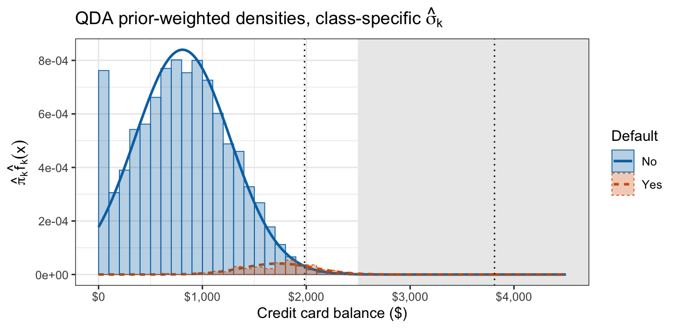

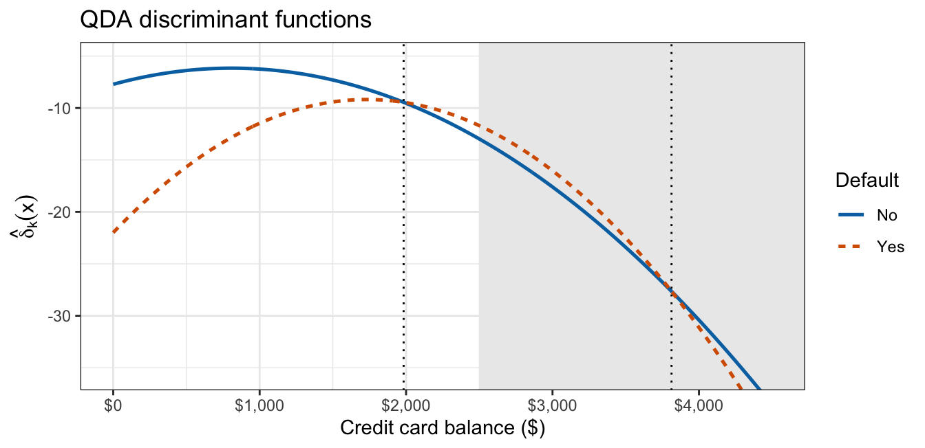
The fitted densities follow the two histograms, apart from the non-defaulters’ spike at zero balance. They cross at $1,984 and again at $3,813, where both are too small to see; the discriminant functions, two downward parabolas, visibly cross a second time. Past that point the wider non-defaulter parabola is the higher one again, so No is assigned in both tails. With the LDA lecture’s one shared standard deviation, the two discriminant functions were straight lines that cross once.

With both features the same happens at every income. The coefficient of $\texttt{balance}^2$ in the table above is negative, because balance varies less among defaulters at a given income, so QDA’s posterior probability of default eventually falls as balance grows. At the lower quartile, median, and upper quartile of training income, $21,297, $34,613, and $43,904, QDA’s posterior crosses $0.5$ at balances of $2,033, $1,969, and $1,918 and again at $3,795, $3,890, and $3,964, beyond the largest training balance, $2,499. The second branch is an extrapolation of the Gaussian tails: no customer in either half has a balance that large.

15.2.5 Bias-variance tradeoff

QDA’s flexibility costs parameters. Not counting the $K - 1$ free priors, which every generative classifier estimates,

\[\text{LDA: } Kp + \frac{p(p+1)}{2}, \qquad \text{QDA: } Kp + K\,\frac{p(p+1)}{2},\]

where

$Kp$ counts the entries of the $K$ mean vectors, and
$p(p+1)/2$ counts the distinct entries of one symmetric $p \times p$ covariance matrix: $p$ variances and $p(p-1)/2$ covariances.

Code

count_lda <- function(K, p) K * p + p * (p + 1) / 2
count_qda <- function(K, p) K * p + K * p * (p + 1) / 2

parameter_table <- tibble(p = c(1, 2, 5, 10, 50)) |>
  mutate(LDA = count_lda(2, p), QDA = count_qda(2, p),
         across(c(LDA, QDA), \(v) format(v, big.mark = ","))) |>
  knitr::kable(col.names = c("Features $p$", "LDA", "QDA"), align = "ccc")

With $K = 2$ classes:

Features $p$	LDA	QDA
1	3	4
2	7	10
5	25	40
10	75	130
50	1,375	2,650

(The previous lecture’s count of 8 for LDA with balance and income included its one free prior.) QDA’s count grows like $Kp^2/2$, against LDA’s $p^2/2$. When the $\Sigma_k$ really differ, LDA’s shared $\Sigma$ makes its boundary the wrong shape however much data it sees: bias. QDA’s boundary has the right shape, but each of its many covariance estimates comes from one class’s observations and varies from one training set to the next: variance. For the credit card customers, QDA estimates the defaulters’ 3 covariance entries from the 176 training defaulters alone, while LDA’s pooled covariance uses all 5,000 training customers.

Code

mu_a    <- c(0, 0)
mu_b    <- c(1.5, 0.5)
Sigma_a <- matrix(c(1, 0.5, 0.5, 1), nrow = 2)
Sigma_b <- matrix(c(3, -0.6, -0.6, 2), nrow = 2)

rmvnorm2 <- function(n, mu, Sigma) {
  sweep(matrix(rnorm(n * 2), n) %*% chol(Sigma), 2, mu, "+")
}
draw_quadratic <- function(n_k) {
  X <- rbind(rmvnorm2(n_k, mu_a, Sigma_a), rmvnorm2(n_k, mu_b, Sigma_b))
  tibble(y = factor(rep(c("k = 1", "k = 2"), each = n_k)),
         x1 = X[, 1], x2 = X[, 2])
}

grid_fit <- expand_grid(x1 = seq(-3.5, 5.5, length.out = 120),
                        x2 = seq(-3.5, 4, length.out = 110))
bayes_grid <- expand_grid(x1 = seq(-3.5, 5.5, length.out = 220),
                          x2 = seq(-3.5, 4, length.out = 200)) |>
  mutate(qda = log_odds_gauss(x1, x2, mu_a, Sigma_a, mu_b, Sigma_b))

n_k_small <- 25
n_k_large <- 250
n_boundary_reps <- 20

fitted_boundaries <- expand_grid(n_k = c(n_k_small, n_k_large),
                                 rep = seq_len(n_boundary_reps)) |>
  mutate(data = map(n_k, draw_quadratic),
         LDA = map(data, \(d) {
           predict(MASS::lda(y ~ x1 + x2, data = d),
                   newdata = grid_fit)$posterior[, "k = 2"]
         }),
         QDA = map(data, \(d) {
           predict(MASS::qda(y ~ x1 + x2, data = d),
                   newdata = grid_fit)$posterior[, "k = 2"]
         })) |>
  select(-data) |>
  pivot_longer(c(LDA, QDA), names_to = "method", values_to = "p_hat") |>
  mutate(grid = list(grid_fit)) |>
  unnest(c(grid, p_hat))

variability_plot <- function(nk) {
  ggplot(filter(fitted_boundaries, n_k == nk), aes(x = x1, y = x2)) +
    geom_contour(aes(z = p_hat - 0.5, group = rep), breaks = 0,
                 color = "grey55", linewidth = 0.35) +
    geom_contour(data = bayes_grid, aes(z = qda), breaks = 0, color = "black",
                 linewidth = 1.1, linetype = "longdash") +
    facet_wrap(~ method) +
    coord_fixed(xlim = c(-3.5, 5.5), ylim = c(-3.5, 4), expand = FALSE) +
    labs(x = expression(X[1]), y = expression(X[2]),
         title = bquote(paste(.(n_boundary_reps), " fitted boundaries, ",
                              n[k] == .(nk),
                              " per class; Bayes boundary long-dashed")))
}
variability_small <- variability_plot(n_k_small)
variability_large <- variability_plot(n_k_large)
cor_of <- function(S) S[1, 2] / sqrt(S[1, 1] * S[2, 2])

The figure below compares fits from repeated training sets against a known Bayes decision boundary, which the credit card data cannot supply, so it uses simulated data: two classes with known Gaussian densities and equal priors, class 1 with mean $(0, 0)^\top$, unit variances, and correlation 0.50, and class 2 with mean $(1.5, 0.5)^\top$, variances 3 and 2, and correlation -0.24. Each panel overlays the boundaries of LDA (left) or QDA (right) fit to each of 20 training sets (thin grey) on the Bayes decision boundary (thick black, long dashes), the QDA boundary computed from the true parameters. The first tab uses 25 observations per class and the second 250.

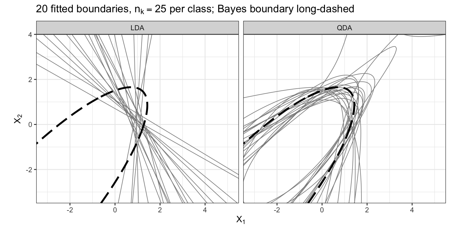
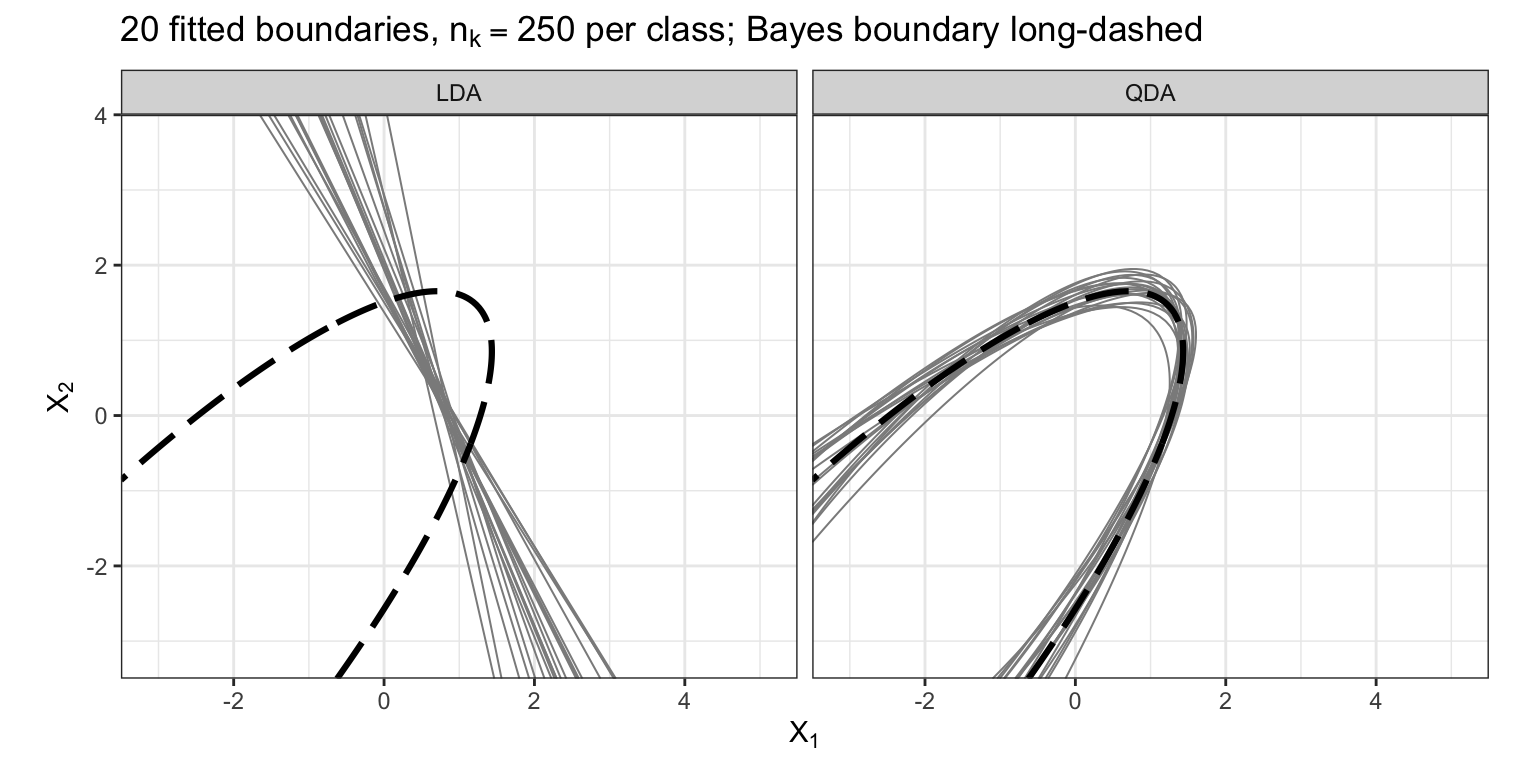
With the small training sets the LDA lines vary in angle and none follows the curvature of the Bayes boundary, while the QDA curves follow its shape but scatter widely. With the large ones the LDA lines tighten around a single line that still misses the curvature, while the QDA curves collapse onto the Bayes boundary: more data reduces QDA’s variance but not LDA’s bias. LDA should therefore win when the training set is small relative to the number of covariance parameters or the class covariance matrices are close to equal, and QDA when they clearly differ and the training set is large enough to estimate them.

Beyond this course

Regularized discriminant analysis compromises between the two by shrinking each class covariance toward the pooled one, $\hat\Sigma_k(\alpha) = \alpha\hat\Sigma_k + (1 - \alpha)\hat\Sigma$, where $\alpha = 0$ gives LDA and $\alpha = 1$ gives QDA. The value of $\alpha$ is a flexibility dial chosen from the data, as the next unit will choose the number of neighbors for KNN.

15.3 Naive Bayes

The figure below shows the training scatterplot once more, points colored and shaped by default status, with each class’s approximately 95% normal-theory ellipse (solid for non-defaulters, dashed for defaulters).

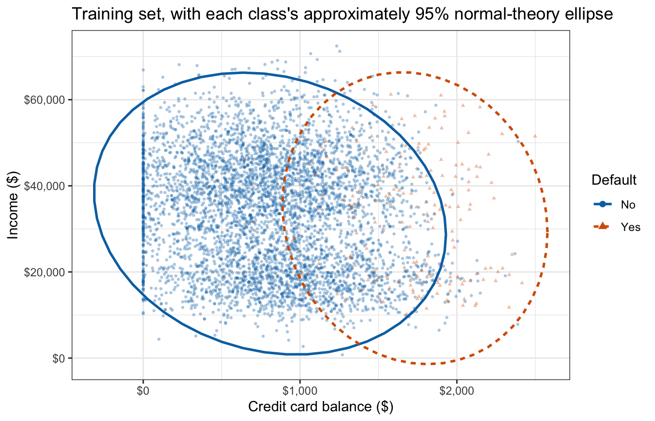
The ellipses tilt only slightly: the within-class correlations are $-0.150$ and $-0.096$, both small in magnitude. A model that treats balance and income as independent within each class ignores only that tilt.

15.3.1 Conditional independence

Naive Bayes keeps the generative framework but replaces the multivariate model for $f_k$ with an assumption about how the features relate to one another:

\[Y_i \stackrel{ind}{\sim} \text{Categorical}\left(\pi_1, \ldots, \pi_K\right), \qquad X_{ij} \mid Y_i = k \stackrel{ind}{\sim} f_{kj}, \qquad i = 1, \ldots, n, \quad j = 1, \ldots, p,\]

where

$Y_i$ and $\text{Categorical}\left(\pi_1, \ldots, \pi_K\right)$ are as in QDA,
$X_{ij}$ is feature $j$ of observation $i$, the $j$th entry of $X_i$,
$f_{kj}$ is the one-feature density (or probability mass function) of feature $j$ among observations in class $k$, and
$\stackrel{ind}{\sim}$ runs over both indices: given $Y_1, \ldots, Y_n$, the $X_{ij}$ are independent over observations $i$ and over features $j$.

Independence over observations is the assumption LDA and QDA also make. Independence over features within an observation, given its class, is the naive assumption that gives the method its name; LDA and QDA instead let the features of one observation be correlated through $\Sigma$ or $\Sigma_k$.

Independence over $j$ turns the joint density of $X_i$ given $Y_i = k$ into the product of its marginals, so the class-conditional density at a value $x = (x_1, \ldots, x_p)^\top$ is

\[f_k(x) = f_{k1}(x_1) \times f_{k2}(x_2) \times \cdots \times f_{kp}(x_p) = \prod_{j=1}^p f_{kj}(x_j).\]

The posterior probability is Bayes’ theorem with this product in place of $f_k(x)$. The assumption is conditional on the class: features that are related only because both differ between classes can be independent within each class while being correlated overall.

Each $f_{kj}$ describes a single feature in a single class, so each can be modeled and estimated separately, and features of different types can use densities of different types.

A quantitative feature is usually modeled as Gaussian, $X_{ij} \mid Y_i = k \stackrel{ind}{\sim} N\left(\mu_{kj}, \sigma_{kj}^2\right)$, with $\mu_{kj}$ and $\sigma_{kj}^2$ estimated by the sample mean and variance of feature $j$ among the class-$k$ training observations.
A binary feature is Bernoulli, $X_{ij} \mid Y_i = k \stackrel{ind}{\sim} \text{Bernoulli}\left(\theta_{kj}\right)$, with $f_{kj}(x_j) = \theta_{kj}^{x_j}\left(1 - \theta_{kj}\right)^{1 - x_j}$ for $x_j \in \{0, 1\}$, where $\theta_{kj} = P(X_{ij} = 1 \mid Y_i = k)$ is estimated by the proportion of class-$k$ training observations with $x_{ij} = 1$.
A categorical feature with $M_j > 2$ levels, coded $1, \ldots, M_j$, gets one probability per level in each class, $X_{ij} \mid Y_i = k \stackrel{ind}{\sim} \text{Categorical}\left(\theta_{kj1}, \ldots, \theta_{kjM_j}\right)$, where $\theta_{kjm} = P(X_{ij} = m \mid Y_i = k)$ is estimated by the proportion of class-$k$ training observations at level $m$.

15.3.2 Naive Bayes fit

e1071::naiveBayes() takes the same formula and models each numeric explanatory variable with a Gaussian density in each class. Fitting it to the training half:

default_nb <- e1071::naiveBayes(default ~ balance + income, data = train)
default_nb


Naive Bayes Classifier for Discrete Predictors

Call:
naiveBayes.default(x = X, y = Y, laplace = laplace)

A-priori probabilities:
Y
    No    Yes 
0.9648 0.0352 

Conditional probabilities:
     balance
Y          [,1]     [,2]
  No   808.2541 458.3208
  Yes 1732.5500 342.2770

     income
Y         [,1]     [,2]
  No  33549.49 13369.50
  Yes 32482.56 13731.38

The header “Naive Bayes Classifier for Discrete Predictors” is e1071’s fixed label, printed although both features here are continuous. The A-priori probabilities are $\hat\pi_k$, the same as QDA’s. Under Conditional probabilities, the balance and income tables give each class’s mean (first column) and standard deviation (second column), the Gaussian $\hat\mu_{kj}$ and $\hat\sigma_{kj}$.

15.3.3 Additive log posterior odds

With $K = 2$, the logarithm of the product is a sum, and the log posterior odds of class $2$ are

\[\log\left[\frac{p_2(x)}{1 - p_2(x)}\right] = \log\frac{\pi_2}{\pi_1} + \sum_{j=1}^p \log\frac{f_{2j}(x_j)}{f_{1j}(x_j)} = \log\frac{\pi_2}{\pi_1} + \sum_{j=1}^p g_j(x_j),\]

where

$g_j(x_j) = \log\left[f_{2j}(x_j)/f_{1j}(x_j)\right]$ is the contribution of feature $j$, a function of $x_j$ alone.

Each feature shifts the log posterior odds by an amount that does not depend on the values of the other features: naive Bayes is an additive model with no interactions, the same structural restriction as the additive logistic regressions of the multiple logistic regression lecture. The form of each $g_j$ follows from the type of $f_{kj}$:

Gaussian with class-specific variances: $g_j$ is quadratic in $x_j$, with coefficient $\frac{1}{2}\left(1/\sigma_{1j}^2 - 1/\sigma_{2j}^2\right)$ on $x_j^2$.
Gaussian with a variance shared by the two classes: the $x_j^2$ terms cancel and $g_j$ is linear in $x_j$.
Bernoulli: $g_j(x_j) = x_j\log\left(\theta_{2j}/\theta_{1j}\right) + \left(1 - x_j\right)\log\left[\left(1 - \theta_{2j}\right)/\left(1 - \theta_{1j}\right)\right]$, linear in $x_j$, so the feature shifts the log posterior odds by $\log\left\{\left[\theta_{2j}/\left(1 - \theta_{2j}\right)\right] / \left[\theta_{1j}/\left(1 - \theta_{1j}\right)\right]\right\}$ when $x_j$ changes from $0$ to $1$.

For the credit card fit both terms are Gaussian with class-specific variances, so the balance term and the income term are each quadratic, and there is no balance-by-income term.

15.3.4 Mixed feature types

A binary feature enters naive Bayes through its own probability table. Adding student as a third feature, naiveBayes() keeps the Gaussian densities for balance and income and estimates, for each class, the proportion of students and non-students; its student table is printed below.

mixed_nb <- e1071::naiveBayes(default ~ balance + income + student, data = train)
mixed_nb$tables$student

     student
Y            No       Yes
  No  0.7039801 0.2960199
  Yes 0.6363636 0.3636364

The second column holds $\hat\theta_k$ (the feature index of $\theta_{kj}$ dropped, since student is the only binary feature), the proportion of students among the training customers of class $k$: 0.296 among non-defaulters and 0.364 among defaulters. By the Bernoulli term above, being a student raises the log posterior odds of default by 0.307 at every balance and income. No Gaussian assumption is made for student, but conditional independence still is: the term ignores that students have much lower incomes than non-students.

15.3.5 Diagonal covariance

When every $f_{kj}$ is Gaussian, the naive Bayes model is $X_{ij} \mid Y_i = k \stackrel{ind}{\sim} N\left(\mu_{kj}, \sigma_{kj}^2\right)$ over $i$ and $j$. Given $Y_i = k$, the joint density of $X_i$ is the product of its $p$ independent normal densities, which is a multivariate normal density with a diagonal covariance matrix:

\[\prod_{j=1}^p \frac{1}{\sqrt{2\pi}\,\sigma_{kj}}\exp\left[-\frac{\left(x_j - \mu_{kj}\right)^2}{2\sigma_{kj}^2}\right] = \frac{1}{(2\pi)^{p/2}\left|\Lambda_k\right|^{1/2}}\exp\left[-\frac{1}{2}\left(x - \mu_k\right)^\top \Lambda_k^{-1}\left(x - \mu_k\right)\right],\]

where

$\mu_k = (\mu_{k1}, \ldots, \mu_{kp})^\top$ is the $p$-vector of class-$k$ feature means, and
$\Lambda_k = \text{diag}\left(\sigma_{k1}^2, \ldots, \sigma_{kp}^2\right)$ is the diagonal matrix of class-$k$ feature variances, whose determinant is $\prod_j \sigma_{kj}^2$ and whose inverse is diagonal with entries $1/\sigma_{kj}^2$.

Read from right to left, the identity says that a multivariate normal density with a diagonal covariance matrix factors into one-feature normal densities, so its entries are independent. The two model statements therefore describe the same distribution, and Gaussian naive Bayes is exactly

\[Y_i \stackrel{ind}{\sim} \text{Categorical}\left(\pi_1, \ldots, \pi_K\right), \qquad X_i \mid Y_i = k \stackrel{ind}{\sim} N_p\left(\mu_k, \Lambda_k\right), \qquad i = 1, \ldots, n.\]

The independence over features $j$ in the naive Bayes model appears in this statement as the zero off-diagonal entries of $\Lambda_k$. Gaussian naive Bayes with class-specific variances is therefore QDA with every $\Sigma_k$ restricted to be diagonal, and Gaussian naive Bayes with one variance per feature shared across classes, $\Lambda_k = \Lambda$, is LDA with $\Sigma$ restricted to be diagonal.

Code

nb_sd <- function(k) c(default_nb$tables$balance[k, 2], default_nb$tables$income[k, 2])
max_diff_sd <- max(map_dbl(c("No", "Yes"), \(k) {
  max(abs(nb_sd(k) - sqrt(diag(qda_par[[k]]$Sigma))))
}))

For the credit card customers, the naive Bayes means are QDA’s and its standard deviations are exactly the square roots of the diagonals of QDA’s $\hat\Sigma_k$: $\hat\Lambda_k$ is $\hat\Sigma_k$ with the within-class correlation, $-0.150$ or $-0.096$, set to zero.

15.3.6 Parameter count

Gaussian naive Bayes with class-specific variances estimates $Kp$ means and $Kp$ variances, $2Kp$ parameters, against QDA’s $Kp + Kp(p+1)/2$. With $K = 2$ and $p = 50$ that is 200 parameters against 2,650. The count grows linearly in $p$, and each parameter is estimated from one feature in one class, using all $n_k$ observations of that class. For balance and income, naive Bayes estimates 8 means and standard deviations against QDA’s 10 means and covariance entries.

For $p$ binary features the saving is larger still: a joint probability mass function has $2^p$ cells per class ($2^p - 1$ free probabilities, or 1,048,575 when $p = 20$), most of them never observed in a training set, against naive Bayes’s $p$ Bernoulli probabilities, which sidesteps the curse of dimensionality of the flexibility lecture.

The price is bias whenever the features are dependent within a class, which in practice is almost always. Only the side of the threshold matters, so a biased estimate of $f_k(x)$ can still produce the Bayes classifier’s classifications.

Beyond this course

A quantitative feature need not be modeled as Gaussian. Each $f_{kj}$ can instead be estimated nonparametrically, by a histogram or a kernel density estimate of feature $j$ within class $k$, since each is a one-dimensional density. The naivebayes package offers this option.

15.3.7 Naive Bayes boundary

The figure below draws the naive Bayes boundary (blue, dot-dash) beside the QDA boundary (orange, dotted) over the training customers, non-defaulters as grey circles and defaulters as black triangles, with balances beyond the largest training balance shaded.

Code

nb_cross <- crossings("Naive Bayes")
stopifnot(all(lengths(nb_cross) == 2),
          all(cross_at(nb_cross, 2) > max(train$balance)))
second_all <- c(cross_at(qda_cross, 2), cross_at(nb_cross, 2))
nb_boundary_plot <- boundary_figure(
  c("QDA", "Naive Bayes"),
  "Naive Bayes and QDA boundaries; shading beyond the largest training balance",
  second_all)
# How each model's balance threshold moves from the lower to the upper income
# quartile, and the largest gap between the two at the three quartiles.
first_qda <- cross_at(qda_cross, 1)
first_nb  <- cross_at(nb_cross, 1)
tilt <- function(v) if (v[3] < v[1]) "falls" else "rises"
nb_tilt <- if (tilt(first_nb) == tilt(first_qda)) paste("also", tilt(first_nb)) else tilt(first_nb)
max_first_gap <- max(abs(first_qda - first_nb))

# Naive Bayes's income term at the median income, per $1,000, against LDA's
# income slope (pooled-covariance coefficient), per $1,000.
nb_income <- default_nb$tables$income
g_income <- function(x) {
  dnorm(x, nb_income["Yes", 1], nb_income["Yes", 2], log = TRUE) -
    dnorm(x, nb_income["No", 1], nb_income["No", 2], log = TRUE)
}
nb_income_slope <- g_income(median(train$income) + 500) -
  g_income(median(train$income) - 500)
income_gap <- nb_income["Yes", 1] - nb_income["No", 1]
pooled <- Reduce(`+`, map(c("No", "Yes"), \(k) {
  crossprod(scale(X_train[train$default == k, ], scale = FALSE))
})) / (nrow(train) - 2)
mean_diff <- c(diff(default_nb$tables$balance[, 1]), income_gap)
lda_income_slope <- 1000 * solve(pooled, mean_diff)[2]
raises <- function(v) if (v > 0) "raises" else "lowers"
# Two significant digits without rounding a small value to 0.0000.
small_num <- function(v) sig_text(v, 2)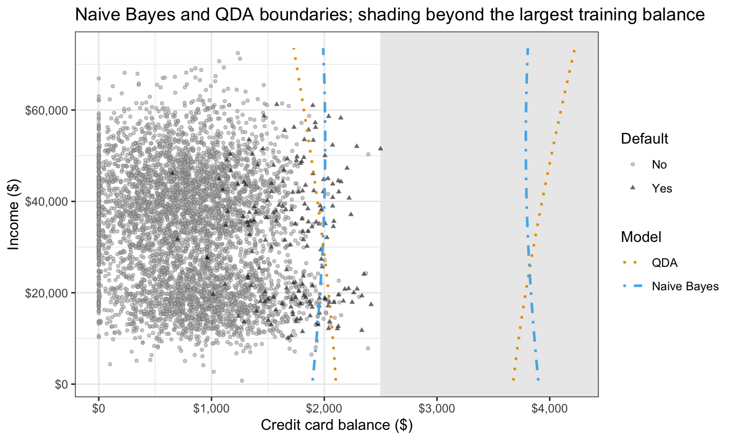

Within the training balances the two boundaries stay within $87 of each other at the three income quartiles. As income rises from the lower to the upper quartile, QDA’s balance threshold falls from $2,033 to $1,918 and naive Bayes’s rises from $1,966 to $2,005. Naive Bayes’s balance term is quadratic for the same reason as QDA’s, so its boundary also has a second branch beyond the training balances, crossing $0.5$ at $3,830, $3,802, and $3,791 at the three income quartiles.

Naive Bayes drops the within-class correlation, so its income term compares the two classes’ income distributions without adjusting for balance: defaulters’ mean training income is $1,067 lower than non-defaulters’, and at the median income each additional $1,000 lowers naive Bayes’s log posterior odds by 0.0053. The term is slightly curved, because the two classes’ income standard deviations differ. LDA’s income slope, adjusted for balance through the pooled within-class covariance as the LDA lecture explained, raises them by 0.017 per $1,000, the opposite direction.

15.4 K-nearest neighbors

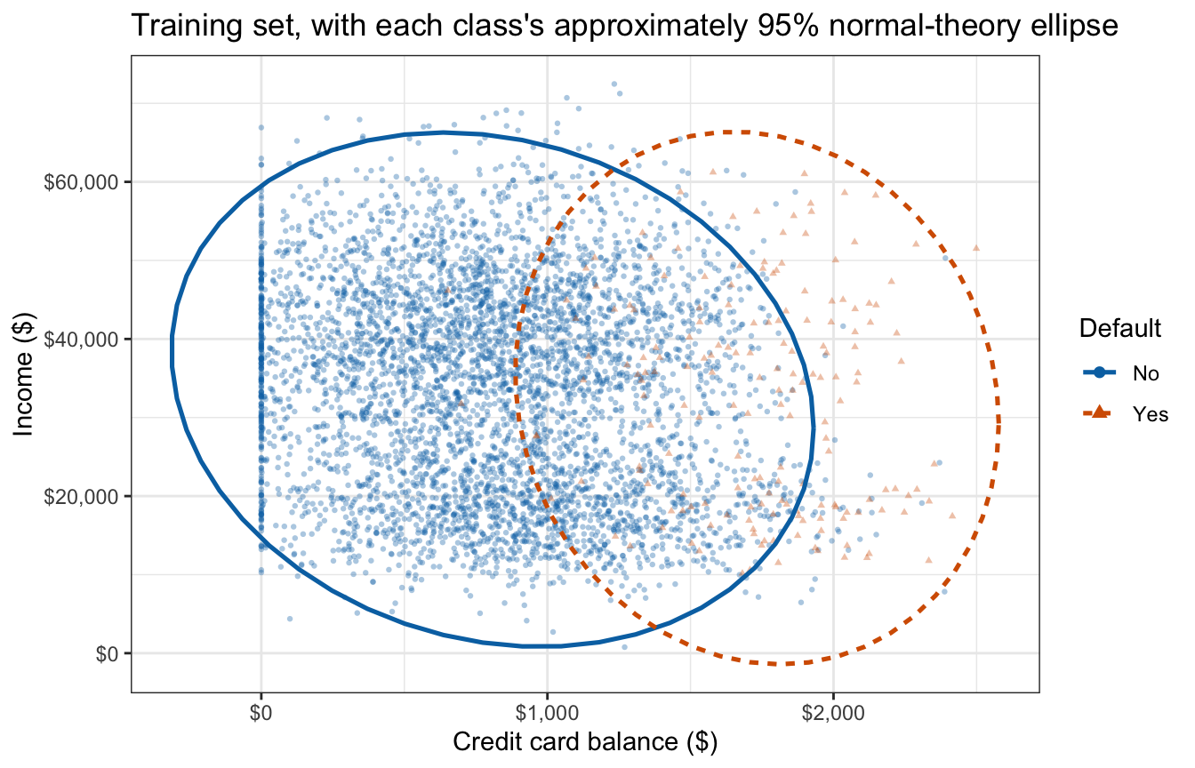
Around any point of the plot, the share of nearby customers who defaulted estimates the probability of default there. That share is near zero at small balances, where almost every customer is a non-defaulter, and rises at the largest balances, where the defaulters sit. K-nearest neighbors (KNN) classifies with that local share directly. It assumes no density for either class, so the ellipses, contours of fitted Gaussian densities, play no part in it.

In this section and the next, $K$ is the number of neighbors rather than the number of classes: every classification in them has two classes, and the number of classes is written as $2$.

15.4.1 Neighbor vote

The flexibility lecture introduced KNN for a quantitative response, averaging the responses of the $K$ nearest training observations. For a qualitative response the $K$ neighbors vote. The estimated probability of class $k$ at a point $x_0$ is the proportion of the $K$ neighbors in class $k$,

\[\hat p_k(x_0) = \frac{1}{K}\sum_{i \in \mathcal{N}_0}\mathrm{I}(y_i = k),\]

where

$x_0$ is the feature vector of the observation being classified,
$k$ indexes the classes, as in the generative classifiers,
$K$ is the number of neighbors, not the number of classes,
$\mathcal{N}_0$ is the set of the $K$ training observations closest to $x_0$ in Euclidean distance after every feature, in the training data and in $x_0$ alike, is standardized by its training mean and standard deviation, since that distance depends on each feature’s scale (as in the flexibility lecture), and
$\mathrm{I}(y_i = k)$ is $1$ when neighbor $i$ is in class $k$ and $0$ otherwise.

The classifier assigns $x_0$ to the class with the largest $\hat p_k(x_0)$, the class most common among its $K$ neighbors, in the same way that the Bayes classifier assigns the class with the largest $p_k(x_0)$. When two or more classes tie for the largest $\hat p_k(x_0)$, a rule is needed to break the tie; class::knn() chooses among the tied classes at random.

For the credit card customers the classes are No and Yes, the feature vector is $x_0 = (\texttt{balance}, \texttt{income})^\top$, and $\hat p_{\text{Yes}}(x_0)$ is the proportion of the $K$ neighbors who defaulted. With two classes, $\hat p_{\text{No}}(x_0) = 1 - \hat p_{\text{Yes}}(x_0)$, so the classifier assigns Yes when $\hat p_{\text{Yes}}(x_0) > 0.5$, a majority of the $K$ neighbors.

15.4.2 Number of neighbors

This lecture fixes the number of neighbors $K$ in advance at the smallest odd integer above $\sqrt{n}$: odd, so that a vote between two classes cannot tie, and near $\sqrt{n}$ as a rule of thumb rather than an optimal choice, since choosing $K$ from the data requires the resampling methods of the next unit. For the credit card training half, $n = 5{,}000$ gives $K = 71$ neighbors.

15.4.3 KNN boundary

The figure below draws the KNN boundary with $K = 71$ neighbors (black, long-and-short dashes) over the training customers, non-defaulters as grey circles and defaulters as black triangles, with balances beyond the largest training balance shaded.

Code

k_default <- odd_above_sqrt(nrow(train))

# KNN vote proportion for "Yes", on features standardized by training means/SDs.
standardize <- function(d) {
  cbind((d$balance - mean(train$balance)) / sd(train$balance),
        (d$income - mean(train$income)) / sd(train$income))
}
knn_yes <- function(target, K) {
  fit <- class::knn(standardize(train), standardize(target), train$default,
                    k = K, prob = TRUE)
  ifelse(fit == "Yes", attr(fit, "prob"), 1 - attr(fit, "prob"))
}

# class::knn() breaks vote ties at random; restoring the generator's state
# keeps this extra figure from changing any later random draw.
rng_state <- .Random.seed
knn_boundary_plot <- boundary_figure(
  "KNN", "KNN boundary; shading beyond the largest training balance",
  second_all)
assign(".Random.seed", rng_state, envir = globalenv())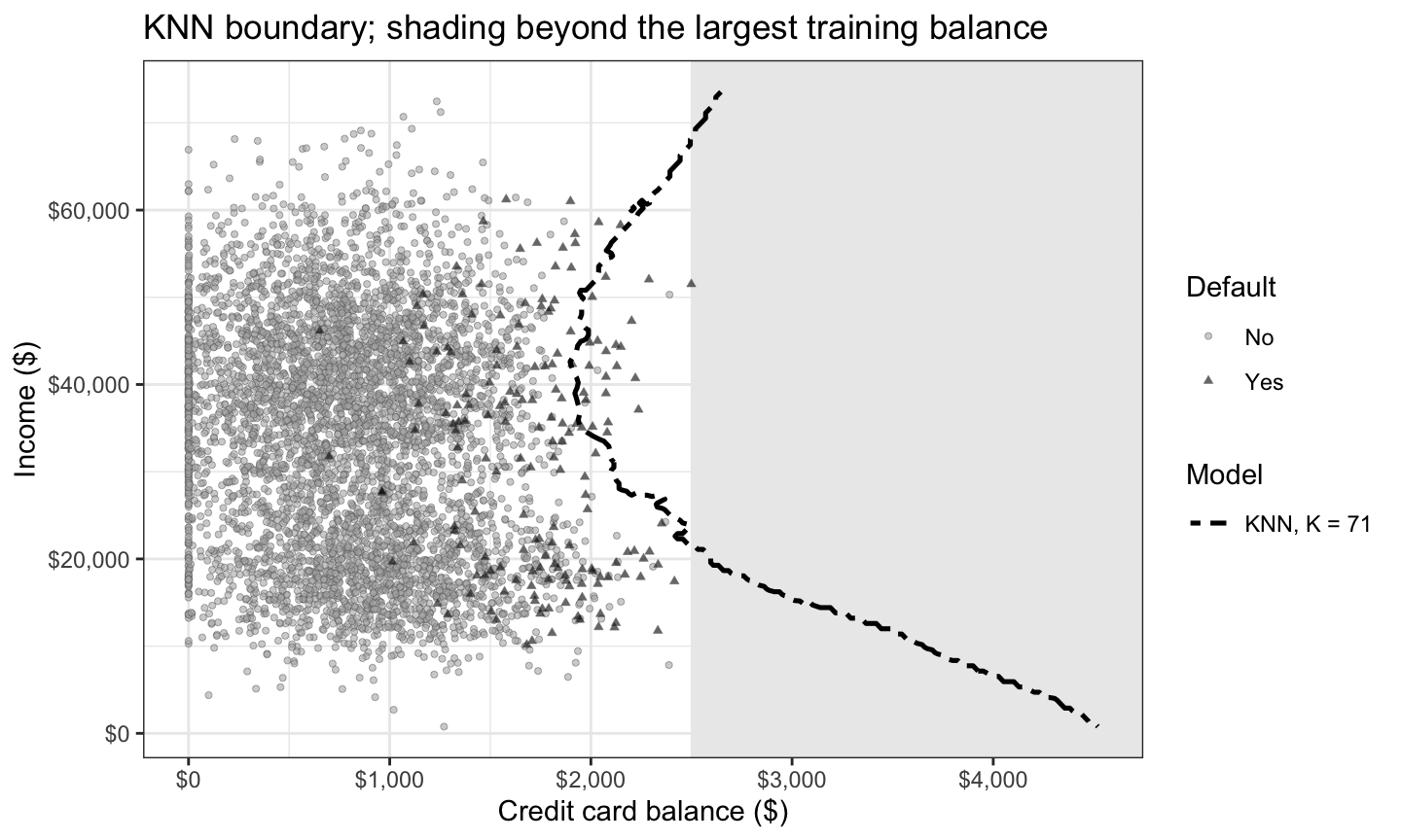

The boundary follows no formula. It is a jagged curve traced by the vote of the nearest training customers, and beyond the largest training balance it is still a vote among the same customers at the edge of the data.

class::knn() fits and classifies in one call. It takes the standardized training features, the standardized features of the customers to classify, the training classes, and the number of neighbors k; with prob = TRUE it also returns the winning class’s share of the vote. The chunk below classifies three customers with the same income and increasing balances.

new_customers <- tibble(balance = c(1000, 2000, 2500), income = 40000)
knn_new <- class::knn(train = standardize(train),
                      test = standardize(new_customers),
                      cl = train$default, k = k_default, prob = TRUE)
knn_new

[1] No  Yes Yes
attr(,"prob")
[1] 1.0000000 0.5352113 0.7183099
Levels: No Yes

At an income of $40,000, the classes and vote shares are No (a vote share of 1.000) at $1,000, Yes (a vote share of 0.535) at $2,000 and Yes (a vote share of 0.718) at $2,500 of balance. The estimate $\hat p_{\text{Yes}}(x_0)$ is the vote share when the class is Yes and one minus it when the class is No.

15.5 Classifier comparison

Five classifiers are now available: logistic regression, LDA, QDA, naive Bayes, and KNN, each compared here on two classes.

15.5.1 Fitted boundaries

Code

default_glm <- glm(default ~ balance + income, data = train,
                   family = "binomial")
all_boundaries_plot <- boundary_figure(
  c("Logistic regression", "LDA", "QDA", "Naive Bayes", "KNN"),
  "All five classifiers' boundaries; shading beyond the largest training balance",
  second_all)

# Incomes (in $1,000 steps) at which KNN flags no balance up to the largest
# training balance, as runs of consecutive grid incomes.
knn_check <- expand_grid(
  income = seq(1000 * floor(min(train$income) / 1000),
               1000 * ceiling(max(train$income) / 1000), by = 1000),
  balance = seq(0, max(train$balance), length.out = 200))
knn_check$yes <- knn_yes(knn_check, k_default) > 0.5
no_flag <- knn_check |>
  group_by(income) |>
  summarize(none = !any(yes), .groups = "drop")
runs <- rle(no_flag$none)
run_end <- cumsum(runs$lengths)
run_start <- run_end - runs$lengths + 1
# Run ends are clipped to the range of training incomes.
no_flag_runs <- tibble(from = pmax(no_flag$income[run_start[runs$values]],
                                   min(train$income)),
                       to = pmin(no_flag$income[run_end[runs$values]],
                                 max(train$income))) |>
  filter(from <= to)
range_text <- function(a, b) {
  if (a == b) paste("near", dollar_text(a)) else
    paste("from", dollar_text(a), "to", dollar_text(b))
}
no_flag_text <- if (nrow(no_flag_runs) == 0) "nowhere" else
  and_list(map2_chr(no_flag_runs$from, no_flag_runs$to, range_text))
# Training defaulters with incomes in those ranges (within $500 of a grid
# income), none of whom KNN flags.
in_no_flag <- map_lgl(train$income, \(v) {
  any(no_flag$none & abs(no_flag$income - v) <= 500)
})
n_def_unflagged <- sum(train$default == "Yes" & in_no_flag)
where_text <- if (nrow(no_flag_runs) == 1) "that range" else "those ranges"
defaulters_text <- if (n_def_unflagged == 0) {
  paste0(", although no training defaulter has an income in ", where_text)
} else if (n_def_unflagged == 1) {
  paste0(", including the one training defaulter with an income in ", where_text)
} else {
  paste0(", including the ", n_def_unflagged,
         " training defaulters with incomes in ", where_text)
}

The figure below shows the training data with every classifier’s fitted 0.5 boundary: non-defaulters as grey circles and defaulters as black triangles, with balances beyond the largest training balance shaded, and logistic regression (with balance and income as its features) pink dashed, LDA green solid, QDA orange dotted, naive Bayes blue dot-dash, and KNN with $K = 71$ neighbors black long-and-short dashes.

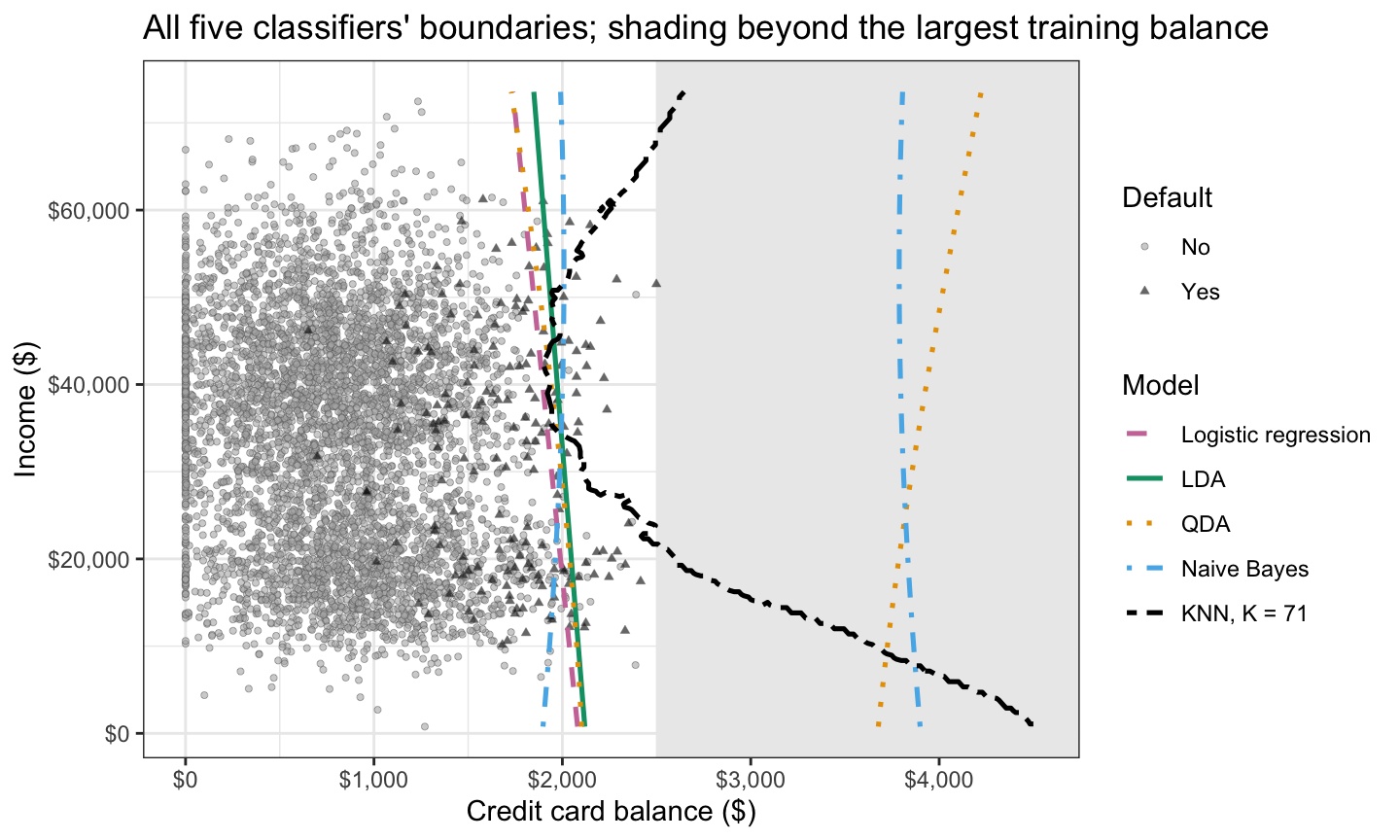
At middle incomes, near the balances where most training defaulters sit, the five boundaries lie close together. The logistic regression and LDA boundaries are straight lines. The QDA and naive Bayes boundaries curve, and each has a second branch beyond the training balances, an extrapolation of their Gaussian tails. The KNN boundary is the jagged curve of the KNN boundary figure. On this split, at incomes from $772 to $21,000 and from $69,000 to $72,461 its threshold lies beyond every training balance, so it flags no customer there, including the 57 training defaulters with incomes in those ranges.

15.5.2 Boundary shapes

With two classes, the log posterior odds derived for the three generative classifiers have the forms

\[\begin{aligned} \text{LDA: } & \beta_0 + \sum_{j=1}^p \beta_j x_j, \\ \text{QDA: } & \beta_0 + \sum_{j=1}^p \beta_j x_j + \sum_{j \le l} \gamma_{jl} x_j x_l, \\ \text{Gaussian naive Bayes: } & \beta_0 + \sum_{j=1}^p \left(\beta_j x_j + \gamma_{jj} x_j^2\right), \end{aligned}\]

where

$\beta_0$ is an intercept and $\beta_j$ the coefficient of $x_j$, with values that differ from method to method, and
$\gamma_{jl}$ is the coefficient of the product $x_j x_l$, a square when $l = j$; for naive Bayes, $\gamma_{jj} = \frac{1}{2}\left(1/\sigma_{1j}^2 - 1/\sigma_{2j}^2\right)$, which is zero when the two classes share feature $j$’s variance.

LDA’s log odds are linear in $x$, and QDA’s are quadratic, with squares and cross-products. Gaussian naive Bayes’s are additive in the features: quadratic in each feature, with squares but no cross-products, when the class variances differ, and linear, LDA’s form, when every variance is shared. A naive Bayes classifier with Bernoulli or categorical features adds terms linear in those features’ indicators. KNN has no formula for its log posterior odds, and its boundary can take any shape.

Logistic regression’s log odds are linear in whatever features it is given. Given $x_1, \ldots, x_p$ it has LDA’s form; given the squares $x_j^2$ as well, Gaussian naive Bayes’s form; and given the cross-products $x_j x_l$ too, as in the flexible logistic regression lecture, QDA’s form. Each generative classifier and the logistic regression of the same form can produce exactly the same set of boundaries. The table pairs them, with each method’s count of free parameters for two classes (for the generative classifiers, the means, variances, covariances, and one free prior). Below each formula, in parentheses, is its value for $p = 2$, the two features of the credit card data.

Code

# Free parameters for two classes, priors included, and logistic regression
# coefficients, intercept included.
# The count for p = 2 goes on its own line, below the formula.
count_with_p2 <- function(formula_tex, f) sprintf("%s<br>(%d)", formula_tex, f(2))
pair_table <- tibble(
  form = c("Linear", "Additive, quadratic in each feature", "Quadratic"),
  generative = c("LDA", "Gaussian naive Bayes", "QDA"),
  gen_count = c(count_with_p2("$1 + 2p + p(p+1)/2$", \(p) 1 + count_lda(2, p)),
                count_with_p2("$1 + 4p$", \(p) 1 + 4 * p),
                count_with_p2("$1 + 2p + p(p+1)$", \(p) 1 + count_qda(2, p))),
  features = c("$x_j$", "$x_j$, $x_j^2$", "$x_j$, $x_j^2$, $x_j x_l$"),
  glm_count = c(count_with_p2("$1 + p$", \(p) 1 + p),
                count_with_p2("$1 + 2p$", \(p) 1 + 2 * p),
                count_with_p2("$1 + p + p(p+1)/2$", \(p) 1 + p + p * (p + 1) / 2))
) |>
  knitr::kable(col.names = c("Log-odds form", "Generative classifier",
                             "Its parameters", "Logistic regression features",
                             "Its coefficients"),
               align = "llccc")

Log-odds form	Generative classifier	Its parameters	Logistic regression features	Its coefficients
Linear	LDA	$1 + 2p + p(p+1)/2$ (8)	$x_j$	$1 + p$ (3)
Additive, quadratic in each feature	Gaussian naive Bayes	$1 + 4p$ (9)	$x_j$, $x_j^2$	$1 + 2p$ (5)
Quadratic	QDA	$1 + 2p + p(p+1)$ (11)	$x_j$, $x_j^2$, $x_j x_l$	$1 + p + p(p+1)/2$ (6)

For the credit card training half, the tabs below draw each pair’s fitted 0.5 boundary over the training customers, as in the five-classifier figure: LDA beside the logistic regression on balance and income, naive Bayes beside the logistic regression that adds $\texttt{balance}^2$ and $\texttt{income}^2$, and QDA beside the logistic regression that also adds $\texttt{balance} \times \texttt{income}$.

Code

squares_glm <- glm(default ~ balance + income + I(balance^2) + I(income^2),
                   data = train, family = "binomial")
quadratic_glm <- glm(default ~ balance + income + I(balance^2) + I(income^2) +
                       balance:income, data = train, family = "binomial")

pairs <- list(
  Linear    = c("LDA", "Logistic regression"),
  Squares   = c("Naive Bayes", "Logistic regression, squares"),
  Quadratic = c("QDA", "Logistic regression, squares and product"))
pair_titles <- c(
  Linear    = "Linear log odds: LDA and logistic regression",
  Squares   = "Squares: naive Bayes and logistic regression",
  Quadratic = "Squares and product: QDA and logistic regression")
# One balance range for all three tabs, the range of boundary_figure()'s grid,
# and the legend below the panel so the panel has the same width in every tab.
pair_xmax <- max(4500, 1.15 * max(second_all))
pair_plots <- imap(pairs, \(m, nm) {
  boundary_figure(m, pair_titles[[nm]], second_all) +
    expand_limits(x = c(0, pair_xmax)) +
    theme(legend.position = "bottom")
})

# Crossings of 0.5 at the three training income quartiles, balances up to
# search_max, and the largest gap between each pair's first crossings.
# predict() for a MASS fit breaks near-ties between classes at random, and
# uniroot() evaluates it at near-ties; restoring the generator's state keeps
# these extra predictions from changing the simulation below.
rng_state <- .Random.seed
pair_cross <- map(pairs, \(m) map(m, crossings))
assign(".Random.seed", rng_state, envir = globalenv())
pair_gap <- map_dbl(pair_cross, \(cr) {
  max(abs(cross_at(cr[[1]], 1) - cross_at(cr[[2]], 1)))
})

# The logistic regressions searched further, to glm_search_max, for a second
# crossing.
glm_search_max <- 30000
glm_cross <- map(c(Squares = "Logistic regression, squares",
                   Quadratic = "Logistic regression, squares and product"),
                 \(m) crossings(m, glm_search_max))
# Coefficient of balance^2 in each model's log posterior odds: for naive
# Bayes, (1/sigma_No^2 - 1/sigma_Yes^2) / 2 from its balance standard
# deviations.
nb_balance <- default_nb$tables$balance
balance_sq <- c(
  QDA = balance_sq_coef,
  `Naive Bayes` = unname(0.5 * (1 / nb_balance["No", 2]^2 -
                                  1 / nb_balance["Yes", 2]^2)),
  Squares = unname(coef(squares_glm)["I(balance^2)"]),
  Quadratic = unname(coef(quadratic_glm)["I(balance^2)"]))
# The prose says: negative balance^2 coefficients for QDA, naive Bayes, and the
# logistic regression with squares, which crosses 0.5 twice at every income
# quartile; a positive one for the logistic regression with squares and
# product, which crosses once and, its log odds rising past that crossing,
# never crosses back.
stopifnot(balance_sq[c("QDA", "Naive Bayes", "Squares")] < 0,
          balance_sq["Quadratic"] > 0,
          all(lengths(glm_cross$Squares) == 2),
          all(lengths(glm_cross$Quadratic) == 1))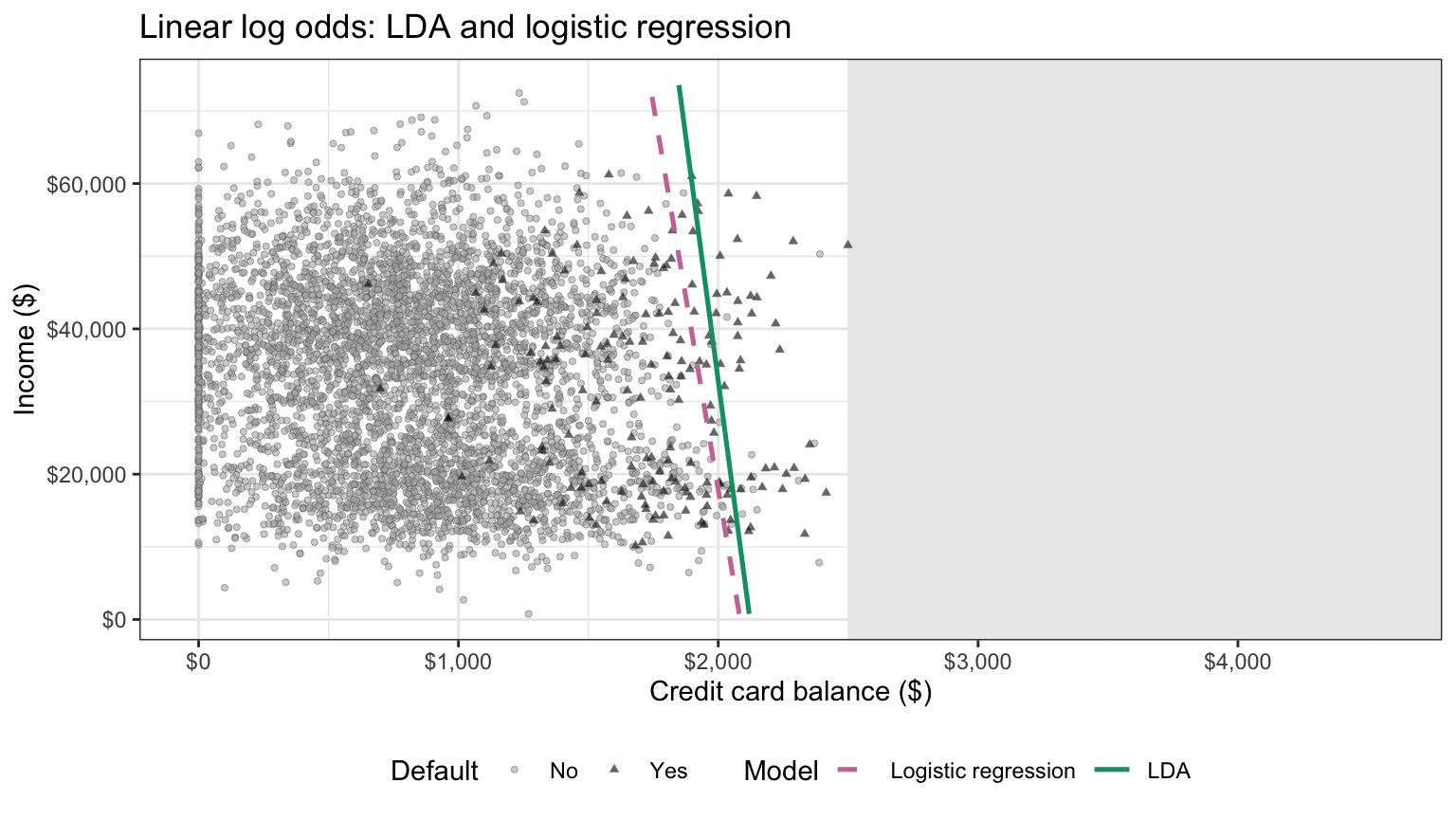

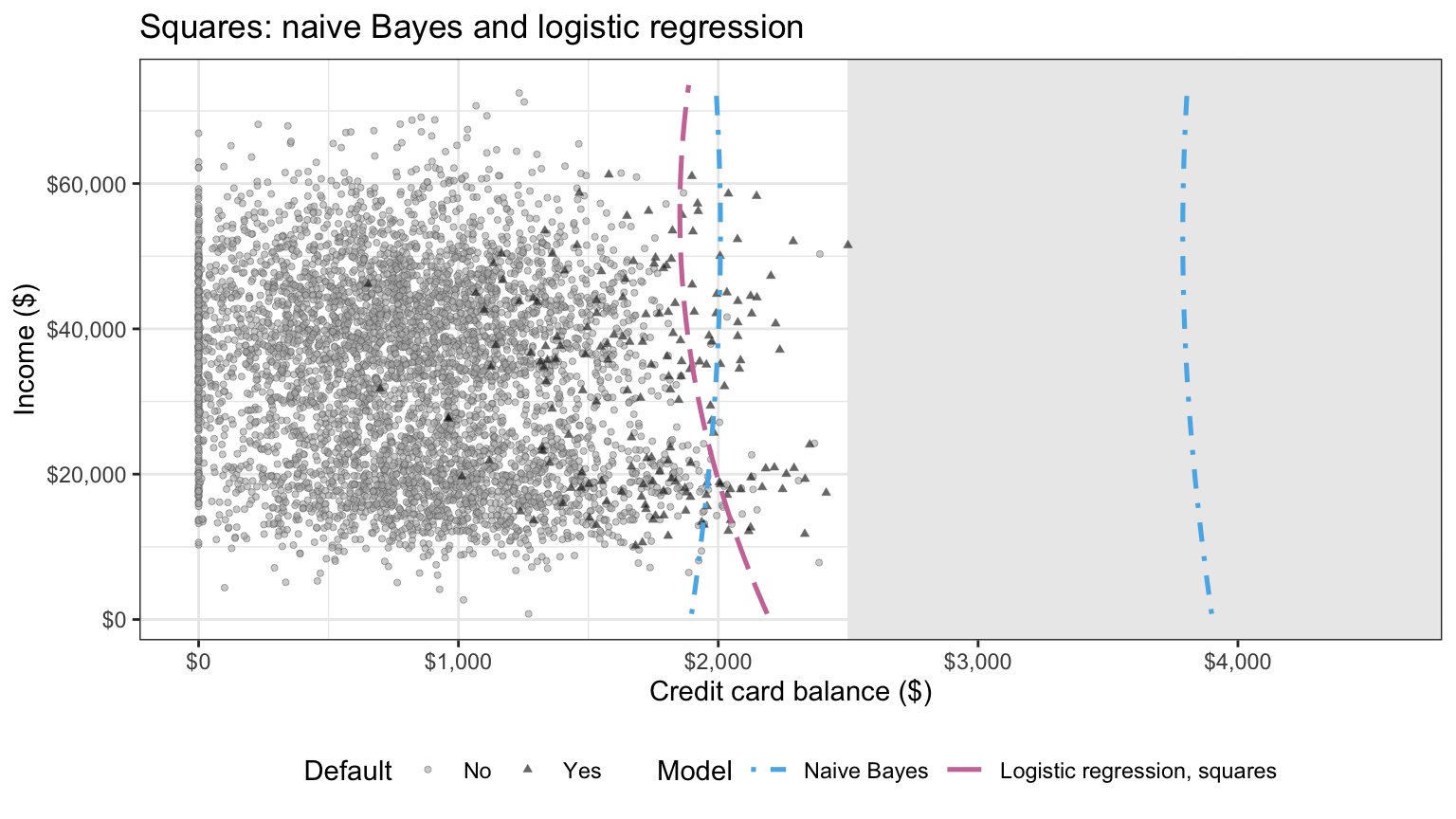
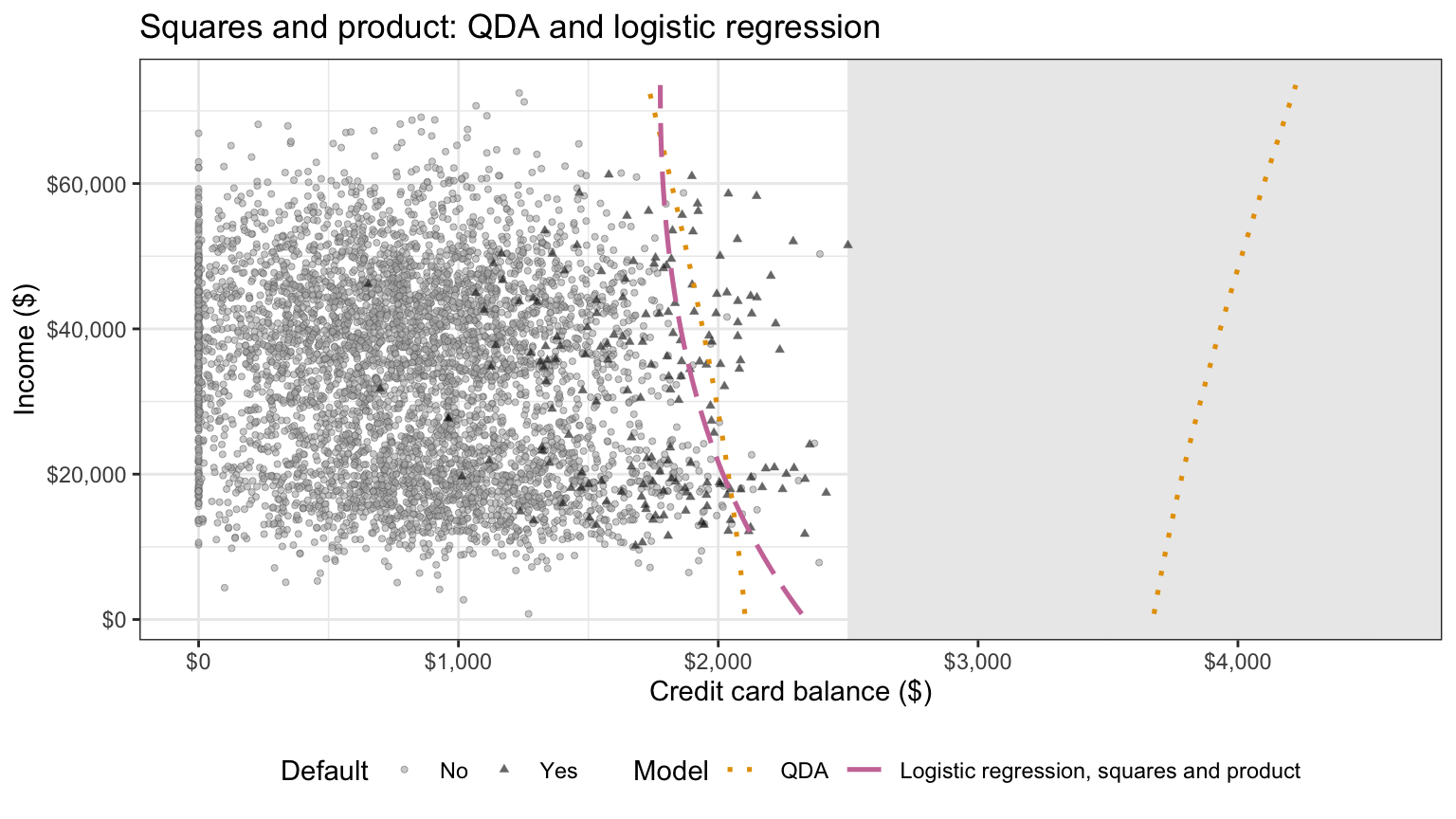
At the lower quartile, median, and upper quartile of training income, the two boundaries of a pair cross $0.5$ at balances within $81 of each other in the linear tab, $137 in the squares tab, and $82 in the squares-and-product tab.

Beyond the training balances, where no training customer constrains either fit, the pairs part. Naive Bayes and the logistic regression with squares both have a negative coefficient of $\texttt{balance}^2$, so both posteriors eventually fall back below $0.5$, but at the median training income naive Bayes crosses $0.5$ again at $3,802 and the logistic regression only at $21,887. QDA’s coefficient of $\texttt{balance}^2$ is negative and that of the logistic regression with squares and product positive, so only QDA crosses back.

The difference within each pair is not in the boundaries the two can represent but in how their parameters are estimated. A generative classifier estimates the class means, variances, covariances, and priors from the joint likelihood of features and responses, in closed form, and computes the log-odds coefficients from them; it has more free parameters than its log odds have coefficients, because it also describes the features’ distribution within each class. Logistic regression estimates the coefficients directly from the conditional likelihood of the responses given the features. When the Gaussian assumptions hold, the generative estimates use that information about the features, which logistic regression ignores; when they fail, the generative coefficients are biased, while logistic regression’s still estimate the log odds, provided its form is correct. The table summarizes the assumptions and estimation of all five classifiers.

Code

comparison_table <- tibble(
  Method = c("Logistic regression", "LDA", "QDA", "Gaussian naive Bayes",
             "KNN"),
  Assumption = c("Log odds linear in its features",
                 "Gaussian, shared covariance",
                 "Gaussian, class covariances",
                 "Gaussian features independent within each class",
                 "Smooth class probabilities"),
  Estimation = c("Conditional likelihood, iterative",
                 "Joint likelihood, closed form",
                 "Joint likelihood, closed form",
                 "Joint likelihood, closed form",
                 "None (stores data)")
) |>
  knitr::kable(align = "lll")

Method	Assumption	Estimation
Logistic regression	Log odds linear in its features	Conditional likelihood, iterative
LDA	Gaussian, shared covariance	Joint likelihood, closed form
QDA	Gaussian, class covariances	Joint likelihood, closed form
Gaussian naive Bayes	Gaussian features independent within each class	Joint likelihood, closed form
KNN	Smooth class probabilities	None (stores data)

KNN is nonparametric, with flexibility set by $1/K$ for $K$ neighbors: it can follow any boundary given enough data, but it needs $n$ large relative to $p$, suffers most from the curse of dimensionality, and has no coefficients to interpret.

Increasing $n$ favors the more flexible methods, QDA and KNN, whose lower bias becomes affordable as their variance shrinks. Increasing $p$ favors the more restricted ones: naive Bayes, whose parameter count grows linearly in $p$, and LDA, whose count grows like $p^2/2$ rather than like QDA’s $p^2$ for two classes.

15.5.3 Simulated scenarios

A small simulation puts these predictions to a test, in four scenarios of two classes with equal priors, each a data-generating process chosen so that a different method’s assumptions hold.

Code

p_indep <- 10                     # independent: number of features
indep_name <- paste0("Independent, p = ", p_indep)
scenario_names <- c("Linear", "Quadratic", indep_name, "Non-linear")
n_reps <- 100       # training sets per scenario
n_train_k <- 50     # training observations per class
n_test_k <- 2000    # test observations per class
k_sim <- odd_above_sqrt(2 * n_train_k)
knn_sim_name <- paste0("KNN, K = ", k_sim)
rho_linear <- 0.5                 # linear: correlation of the shared covariance
mu_linear <- c(1.5, 0.5)          # linear: class 2 mean (class 1 at the origin)
shift_indep <- 0.5                # independent: class 2 mean, first half
var_indep <- 2                    # independent: class 2 variance, second half
flip_rate <- 0.1                  # non-linear: share of labels flipped
S_linear <- matrix(c(1, rho_linear, rho_linear, 1), nrow = 2)
mu_indep <- rep(c(shift_indep, 0), each = p_indep / 2)
var_indep_2 <- rep(c(1, var_indep), each = p_indep / 2)

rmvnorm_p <- function(n, mu, Sigma) {
  sweep(matrix(rnorm(n * length(mu)), n) %*% chol(Sigma), 2, mu, "+")
}

# One data set of 2 * n_k observations, n_k per class (in expectation for the
# non-linear scenario, whose class sizes are random).
draw_scenario <- function(scenario, n_k) {
  labels <- c("Class 1", "Class 2")
  if (scenario == "Non-linear") {
    X <- matrix(runif(4 * n_k, -2, 2), ncol = 2)
    y <- as.numeric(X[, 2] > sin(2 * X[, 1]))
    flip <- runif(2 * n_k) < flip_rate
    y[flip] <- 1 - y[flip]
    y <- factor(labels[y + 1], levels = labels)
  } else {
    if (scenario == "Linear") {
      X <- rbind(rmvnorm_p(n_k, c(0, 0), S_linear),
                 rmvnorm_p(n_k, mu_linear, S_linear))
    }
    if (scenario == "Quadratic") {
      X <- rbind(rmvnorm_p(n_k, mu_a, Sigma_a), rmvnorm_p(n_k, mu_b, Sigma_b))
    }
    if (scenario == indep_name) {
      X <- rbind(rmvnorm_p(n_k, rep(0, p_indep), diag(p_indep)),
                 rmvnorm_p(n_k, mu_indep, diag(var_indep_2)))
    }
    y <- factor(rep(labels, each = n_k), levels = labels)
  }
  colnames(X) <- paste0("x", seq_len(ncol(X)))
  bind_cols(tibble(y = y), as_tibble(X))
}

# Bayes classifier's error rate on a test set, from the true model.
bayes_error <- function(scenario, test) {
  X <- as.matrix(select(test, -y))
  pred <- switch(scenario,
    "Non-linear" = X[, 2] > sin(2 * X[, 1]),
    Linear = log_odds_gauss(X[, 1], X[, 2], c(0, 0), S_linear, mu_linear,
                            S_linear) > 0,
    Quadratic = log_odds_gauss(X[, 1], X[, 2], mu_a, Sigma_a, mu_b, Sigma_b) > 0,
    rowSums(dnorm(X, mu_indep[col(X)], sqrt(var_indep_2)[col(X)], log = TRUE) -
              dnorm(X, log = TRUE)) > 0)
  mean(pred != (test$y == "Class 2"))
}

# Test error rate of each method fit to one training set; KNN uses features
# standardized by the training means and SDs.
fit_methods <- function(train, test) {
  truth <- test$y
  X_train <- as.matrix(select(train, -y))
  Z_train <- scale(X_train)
  Z_test  <- scale(as.matrix(select(test, -y)), attr(Z_train, "scaled:center"),
                   attr(Z_train, "scaled:scale"))
  knn_error <- function(K) mean(class::knn(Z_train, Z_test, train$y, k = K) != truth)
  p_glm <- predict(glm(y ~ ., data = train, family = "binomial"), test,
                   type = "response")
  c(`Logistic regression` = mean((p_glm > 0.5) != (truth == "Class 2")),
    LDA = mean(predict(MASS::lda(y ~ ., data = train), test)$class != truth),
    QDA = mean(predict(MASS::qda(y ~ ., data = train), test)$class != truth),
    `Naive Bayes` = mean(predict(e1071::naiveBayes(y ~ ., data = train), test) != truth),
    `KNN, K = 1` = knn_error(1)) |>
    c(setNames(knn_error(odd_above_sqrt(nrow(train))), knn_sim_name))
}

scenario_results <- map(scenario_names, \(s) {
  test <- draw_scenario(s, n_test_k)
  errors <- map(seq_len(n_reps),
                \(r) fit_methods(draw_scenario(s, n_train_k), test))
  list(errors = bind_rows(errors) |> mutate(scenario = s, rep = row_number()),
       bayes = bayes_error(s, test))
})

method_levels <- c("Logistic regression", "LDA", "QDA", "Naive Bayes",
                   "KNN, K = 1", knn_sim_name)

scenario_errors <- map(scenario_results, "errors") |>
  bind_rows() |>
  pivot_longer(all_of(method_levels), names_to = "method",
               values_to = "error") |>
  mutate(method = factor(method, levels = method_levels),
         scenario = factor(scenario, levels = scenario_names))

scenario_bayes <- tibble(scenario = factor(scenario_names, levels = scenario_names),
                         bayes = map_dbl(scenario_results, "bayes"))
scenario_means <- scenario_errors |>
  group_by(scenario, method) |>
  summarize(mean_error = mean(error), .groups = "drop")
mean_error_of <- function(s, m) {
  with(scenario_means, mean_error[scenario == s & method == m])
}
best_method <- function(s) {
  with(filter(scenario_means, scenario == s), as.character(method[which.min(mean_error)]))
}
pct <- function(v) sprintf("%.1f%%", 100 * v)

# Prose labels for the winning method of each scenario.
prose_label <- setNames(c("logistic regression", "LDA", "QDA", "naive Bayes",
                          "KNN with $K = 1$", paste0("KNN with $K = ", k_sim, "$")),
                        c("Logistic regression", "LDA", "QDA", "Naive Bayes",
                          "KNN, K = 1", knn_sim_name))
winner <- function(s) unname(prose_label[best_method(s)])

pp <- function(v) sprintf("%.3f", 100 * v)   # percentage points

# One training set per scenario to show what the data look like; the
# independent scenario is shown in features 1 (mean shift) and 6 (variance).
scenario_examples <- map(scenario_names, \(s) {
  draw_scenario(s, n_train_k) |>
    transmute(y, first = x1,
              second = if (s == indep_name) .data[[paste0("x", p_indep / 2 + 1)]] else x2,
              scenario = s)
}) |>
  bind_rows() |>
  mutate(scenario = factor(scenario, levels = scenario_names))

scenario_data_plot <- ggplot(scenario_examples,
                             aes(x = first, y = second, color = y, shape = y)) +
  geom_point(size = 1.6, alpha = 0.8) +
  facet_wrap(~ scenario, scales = "free") +
  scale_color_manual(values = class_colors) +
  labs(x = "First plotted feature", y = "Second plotted feature",
       color = "Class", shape = "Class",
       title = paste0("One training set per scenario (Independent: features 1 and ",
                      p_indep / 2 + 1, ")"))

scenario_error_plot <- ggplot(scenario_errors, aes(x = method, y = error)) +
  geom_boxplot(outlier.size = 0.6, fill = "grey90") +
  geom_hline(data = scenario_bayes, aes(yintercept = bayes),
             linetype = "dashed") +
  facet_wrap(~ scenario, scales = "free_y") +
  labs(x = NULL, y = "Test error rate",
       title = paste("Test error rates over", n_reps,
                     "training sets; Bayes error rate dashed")) +
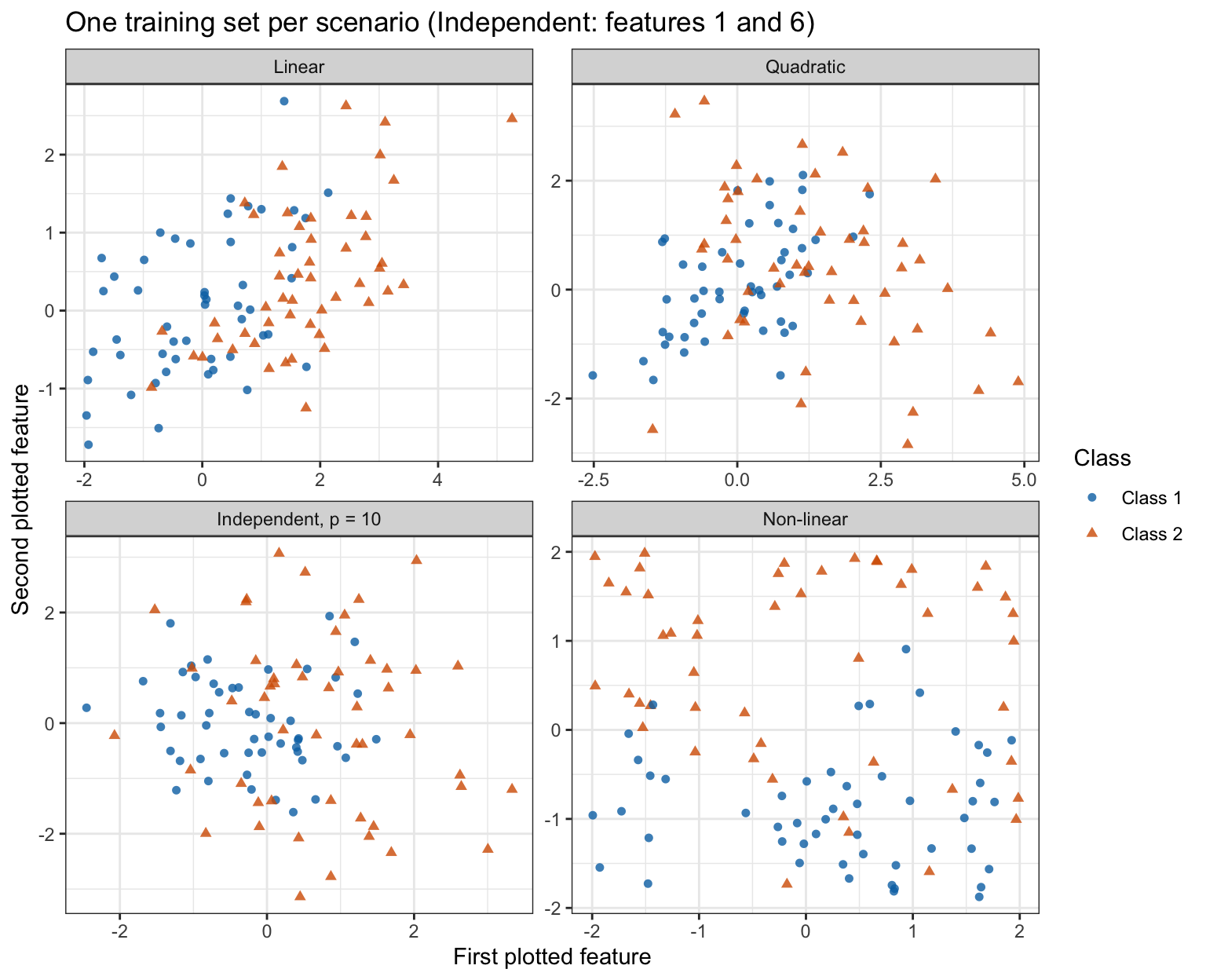
  theme(axis.text.x = element_text(angle = 35, hjust = 1))

Linear: two Gaussian features, a shared covariance matrix with correlation $0.5$, and class means $(0, 0)^\top$ and $(1.5, 0.5)^\top$, so the Bayes boundary is a line.
Quadratic: the two classes of the variability figure, with class-specific covariance matrices.
Independent, $p = 10$: 10 Gaussian features, independent within each class; class 2’s mean is 0.5 in the first 5 features and its variance 2 in the last 5, against means 0 and variances 1 in class 1.
Non-linear: two features uniform on a square, class $2$ above the curve $x_2 = \sin(2x_1)$ and class $1$ below it, and then 10% of the class labels flipped at random, so neither class is Gaussian and the Bayes boundary is the sine curve.

In each scenario, 100 training sets of 100 observations were drawn, 50 per class (in expectation in the non-linear scenario). Each method was fit to every training set and its error rate computed on one large test set of 4,000 observations drawn from the same scenario. KNN was fit on standardized features with $K = 1$ and with $K = 11$, the KNN rule above for the $n = 100$ training observations.

The first tab below shows one training set from each scenario, classes distinguished by color and shape, with features 1 and 6 for the independent scenario. In the second, each box summarizes the test error rates of one method over the 100 training sets, and the dashed line is the Bayes error rate, the floor no classifier can beat on average.

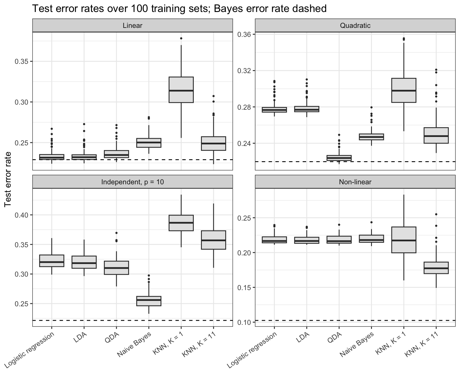
Linear. Logistic regression and LDA both average 23.4%, against a Bayes error rate of 22.9%. QDA, whose extra covariance parameters are unnecessary here, averages 23.7%: with only two features its variance penalty is small. Naive Bayes, which ignores the correlation, averages 25.0%.
Quadratic. QDA’s average of 22.5% beats logistic regression’s 27.9% and LDA’s 27.9%: the linear methods’ bias outweighs QDA’s variance. Naive Bayes, curved but missing the cross-product, falls between them, at 24.8%.
Independent, $p = 10$. Naive Bayes, whose assumption holds exactly, averages 25.6% with 40 parameters. QDA’s model also contains the truth, but it estimates 130 parameters from 100 observations and averages 31.1%. KNN, with 10 dimensions to search for neighbors, averages 35.8% with $K = 11$.
Non-linear. No model-based method can represent a sine curve, and all four average between 21.8% and 22.0%. KNN with $K = 11$ averages 18.0%. With $K = 1$ its variance erases that advantage: it averages 21.8%, about the same as the model-based methods.

In the quadratic, independent, and non-linear scenarios the best method is the one whose assumptions are the most restrictive ones that still hold: QDA in the quadratic, naive Bayes in the independent, and KNN with $K = 11$ in the non-linear scenario. In the linear scenario both LDA and logistic regression are correct models, and their averages differ by only 0.035 percentage points, with logistic regression ahead: with two features, LDA’s extra assumption buys essentially nothing.

15.5.4 Test performance

Returning to the credit card customers, every classifier of the five-boundary figure, with KNN also at $K = 1$, is scored on both halves.

Code

knn_default_name <- paste0("KNN, K = ", k_default)
model_based_names <- c("Logistic regression", "LDA", "QDA", "Naive Bayes")
all_scores <- function(d) {
  map(model_based_names, \(m) posterior_of(m, d)) |>
    set_names(model_based_names) |>
    as_tibble() |>
    mutate(`KNN, K = 1` = knn_yes(d, 1), "{knn_default_name}" := knn_yes(d, k_default))
}
scores_train <- all_scores(train)
scores_test  <- all_scores(test)

# Empirical ROC curve: every distinct score is a cutoff; classify positive
# when score >= cutoff.
roc_curve <- function(score, positive) {
  ord <- order(score, decreasing = TRUE)
  s   <- score[ord]
  pos <- positive[ord]
  keep <- c(diff(s) != 0, TRUE)
  tibble(fpr = c(0, cumsum(!pos)[keep] / sum(!positive)),
         tpr = c(0, cumsum(pos)[keep] / sum(positive)))
}

# Area under an ROC curve (sorted by fpr) by the trapezoid rule.
auc_trapezoid <- function(roc) {
  with(roc, sum(diff(fpr) * (head(tpr, -1) + tail(tpr, -1)) / 2))
}
yes_train <- train$default == "Yes"
yes_test  <- test$default == "Yes"

rates <- function(p_train, p_test) {
  tibble(train_error = mean((p_train > 0.5) != yes_train),
         test_error  = mean((p_test > 0.5) != yes_test),
         sensitivity = mean(p_test[yes_test] > 0.5),
         specificity = mean(p_test[!yes_test] <= 0.5),
         auc         = auc_trapezoid(roc_curve(p_test, yes_test)),
         flagged     = sum(p_test > 0.5))
}
performance <- map(names(scores_test), \(m) rates(scores_train[[m]], scores_test[[m]])) |>
  set_names(names(scores_test)) |>
  list_rbind(names_to = "model")
perf_of <- function(m, col) performance[[col]][performance$model == m]
model_based <- performance |> slice(1:4)
# Optimism sentence, with a separate wording for each count of model-based
# classifiers whose training error rate is above their test error rate.
n_train_above <- sum(model_based$train_error > model_based$test_error)
chance <- "Training error rates are optimistic on average, but on a single split chance can outweigh that: "
optimism_text <- if (n_train_above == 0) {
  "No model-based classifier has a training error rate above its test error rate, as optimism predicts."
} else if (n_train_above < 4) {
  paste0(chance, c("one of the four model-based classifiers has",
                   "two of the four model-based classifiers have",
                   "three of the four model-based classifiers have")[n_train_above],
         " a training error rate above the test error rate.")
} else {
  paste0(chance, "all four model-based classifiers have a training error rate above ",
         "their test error rate",
         if (n_defaults[["train"]] > n_defaults[["test"]]) sprintf(
           ", perhaps because the training half drew %d defaulters (%s) and the test half %d (%s).",
           n_defaults[["train"]], pct2(mean(yes_train)), n_defaults[["test"]],
           pct2(mean(yes_test))) else ".")
}

performance_table <- performance |>
  select(-flagged) |>
  mutate(across(train_error:specificity, pct2), auc = sprintf("%.4f", auc)) |>
  knitr::kable(col.names = c("Model", "Training error", "Test error",
                             "Test sensitivity", "Test specificity", "Test AUC"),
               align = "lccccc")

# Naive Bayes against QDA, from the rates as displayed in the table.
nb_error_diff <- round(perf_of("Naive Bayes", "test_error") - perf_of("QDA", "test_error"), 4)
nb_auc_diff   <- round(perf_of("Naive Bayes", "auc"), 4) - round(perf_of("QDA", "auc"), 4)
higher_lower <- function(d) if (d > 0) "higher" else "lower"
nb_error_text <- if (nb_error_diff == 0) "the same as QDA's" else
  paste(sprintf("%.2f percentage points", 100 * abs(nb_error_diff)),
        higher_lower(nb_error_diff), "than QDA's")
nb_auc_text <- if (nb_auc_diff == 0) "the same as QDA's" else
  paste(sprintf("%.4f", abs(nb_auc_diff)), higher_lower(nb_auc_diff))
nb_cost <- if (nb_error_diff <= 0 && nb_auc_diff >= 0) "does not hurt naive Bayes" else
  "costs naive Bayes little"

# Model-based classifiers with the highest sensitivity and the most customers
# flagged, named in prose (ties listed together).
model_label <- c(`Logistic regression` = "logistic regression", LDA = "LDA",
                 QDA = "QDA", `Naive Bayes` = "naive Bayes")
top_models <- function(col) {
  v <- round(model_based[[col]], 6)
  unname(model_label[model_based$model[v == max(v)]])
}
sens_top <- top_models("sensitivity")
flag_top <- top_models("flagged")
# "is X's" for one model, "is shared by X and Y" for a tie.
owner <- function(x) if (length(x) == 1) paste0("is ", x, "'s") else paste("is shared by", and_list(x))
top_text <- paste0("The highest sensitivity ", owner(sens_top),
  if (identical(sens_top, flag_top) && length(flag_top) == 1) ", which flags" else
    paste0("; ", and_list(flag_top), if (length(flag_top) == 1) " flags" else " flag"),
  " the most test customers, ", max(model_based$flagged), ".")

# KNN's place among the classifiers, stated only when it holds.
knn1_worst <- perf_of("KNN, K = 1", "test_error") == max(performance$test_error)
knn_auc_lowest <- perf_of(knn_default_name, "auc") < min(model_based$auc)

# The opening question, answered from the table's rounded test error rates.
all_label <- c(model_label, setNames(c("KNN with $K = 1$",
                                       paste0("KNN with $K = ", k_default, "$")),
                                     c("KNN, K = 1", knn_default_name)))
err4 <- setNames(round(performance$test_error, 4), performance$model)
lowest_text <- owner(unname(all_label[names(err4)[err4 == min(err4)]]))
new_vs_old <- min(err4[c("LDA", "Logistic regression")]) - min(err4[c("QDA", "Naive Bayes")])
new_vs_old_text <- if (new_vs_old == 0) "the same as" else
  paste(sprintf("%.2f percentage points", 100 * abs(new_vs_old)),
        if (new_vs_old > 0) "lower than" else "higher than")
knn_best <- min(err4[c("KNN, K = 1", knn_default_name)])
knn_vs_text <- if (knn_best > max(err4[model_based$model])) {
  "both KNN classifiers have higher test error rates than every model-based classifier"
} else if (knn_best < min(err4[model_based$model])) {
  "the better KNN classifier has a lower test error rate than every model-based classifier"
} else {
  "the better KNN classifier's test error rate falls within the model-based classifiers' range"
}

KNN uses $K = 1$ and $K = 71$. The table gives each classifier’s training error rate and its test error rate, sensitivity, and specificity at threshold $0.5$ (for KNN, a majority vote), and test AUC, the measures of the previous lecture.

Model	Training error	Test error	Test sensitivity	Test specificity	Test AUC
Logistic regression	2.78%	2.46%	31.85%	99.67%	0.9551
LDA	2.96%	2.54%	24.84%	99.81%	0.9553
QDA	2.92%	2.52%	27.39%	99.75%	0.9550
Naive Bayes	3.12%	2.46%	28.03%	99.79%	0.9533
KNN, K = 1	0.00%	4.18%	29.94%	97.96%	0.6395
KNN, K = 71	3.12%	2.88%	10.83%	99.92%	0.9326

Training error rates are optimistic on average, but on a single split chance can outweigh that: all four model-based classifiers have a training error rate above their test error rate, perhaps because the training half drew 176 defaulters (3.52%) and the test half 157 (3.14%). KNN with $K = 1$ shows the optimism plainly: its training error rate is 0.00%, since each training customer is its own nearest neighbor, against a test error rate of 4.18%, the worst in the table.

The four model-based classifiers have test error rates between 2.46% and 2.54%, against the 3.14% of predicting No for every test customer. They differ more in sensitivity, from 24.84% to 31.85%, a difference of 11 of the 157 test defaulters. The highest sensitivity is logistic regression’s, which flags the most test customers, 66. Their test AUCs range only from 0.9533 to 0.9553. With the within-class correlation this small, dropping it costs naive Bayes little: its test error rate is 0.06 percentage points lower than QDA’s, and its AUC is 0.0017 lower. KNN with $K = 71$ has a lower test AUC than any of them, 0.9326, and a test sensitivity of 10.83%, below every model-based classifier’s, consistent with the incomes at which its boundary flags no one.

To answer the opening question on this split: the lowest test error rate is shared by logistic regression and naive Bayes; the better of QDA and naive Bayes has a test error rate the same as the better of LDA and logistic regression; and both KNN classifiers have higher test error rates than every model-based classifier.

15.6 Student strata

Student status has entered only the mixed naive Bayes fit, which has not yet been scored on the test half. The table below summarizes the two student strata of the training half, and the figure plots income against balance in each stratum, points colored and shaped by default status, with each panel’s income axis covering its own stratum’s incomes.

Code

strata_summary <- train |>
  group_by(student) |>
  summarize(n = n(), defaulters = sum(default == "Yes"),
            rate = mean(default == "Yes"), median_income = median(income),
            .groups = "drop")
strata_summary_of <- function(s, col) strata_summary[[col]][strata_summary$student == s]
strata_summary_table <- strata_summary |>
  transmute(student, n = format(n, big.mark = ","), defaulters,
            rate = pct2(rate), median_income = dollar_text(median_income)) |>
  knitr::kable(col.names = c("Student", "Customers", "Defaulters",
                             "Default rate", "Median income"), align = "ccccc")
strata_data_plot <- ggplot() +
  scatter_points +
  facet_wrap(~ student, labeller = label_both, scales = "free_y") +
  guides(color = guide_legend(override.aes = list(alpha = 1, size = 2))) +
  labs(title = "Training set, income against balance by student status")

Student	Customers	Defaulters	Default rate	Median income
No	3,508	112	3.19%	$40,135
Yes	1,492	64	4.29%	$17,980

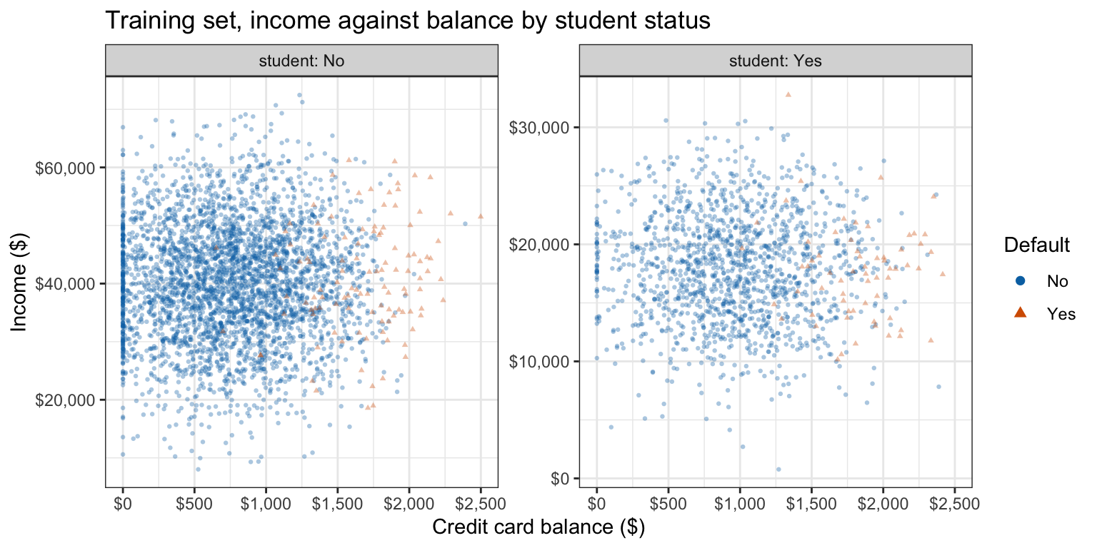
Students default more often, 4.29% against 3.19%, and their incomes occupy a lower band; in both strata the defaulters sit at the larger balances. These numbers differ from the previous lecture’s strata table because that lecture used all customers and this one the training half.

In this additional analysis, QDA with balance and income is fit separately to each stratum, beside the logistic regression whose intercept and slopes all interact with student status. Each stratum’s QDA uses that stratum’s class proportions as priors, so every customer’s score is its posterior probability given balance, income, and student status, on one common scale across strata, which is what lets a single error rate and AUC be computed over all customers.

Naive Bayes can instead take student status as one more feature, as in the mixed feature types fit: a Bernoulli term assumed independent of balance and income given default, so students and non-students share one set of balance and income densities. That fit is set beside the naive Bayes fit with balance and income alone.

Code

strata <- c(No = "No", Yes = "Yes")
train_by <- map(strata, \(s) filter(train, student == s))
strata_qda <- map(train_by, \(d) MASS::qda(default ~ balance + income, data = d))
strata_glm <- map(train_by, \(d) glm(default ~ balance + income, data = d,
                                     family = "binomial"))
interacted_glm <- glm(default ~ (balance + income) * student, data = train,
                      family = "binomial")

# Score every customer with its own stratum's model.
by_stratum <- function(d, score) {
  p <- numeric(nrow(d))
  for (s in strata) p[d$student == s] <- score(s, d[d$student == s, ])
  p
}
qda_strat <- function(d) by_stratum(d, \(s, ds) predict(strata_qda[[s]], ds)$posterior[, "Yes"])
max_diff_int <- max(abs(fitted(interacted_glm) - by_stratum(train, \(s, ds) {
  predict(strata_glm[[s]], ds, type = "response")
})))
glm_int <- function(d) predict(interacted_glm, newdata = d, type = "response")
nb_mixed_yes <- function(d) predict(mixed_nb, newdata = d, type = "raw")[, "Yes"]

# Rates rounded as displayed, so changes computed from them match the table.
strata_rates <- list(
  "QDA, single fit" = rates(scores_train$QDA, scores_test$QDA),
  "QDA, by student stratum" = rates(qda_strat(train), qda_strat(test)),
  "Logistic regression, additive" = rates(scores_train$`Logistic regression`,
                                          scores_test$`Logistic regression`),
  "Logistic regression, interacted with student" =
    rates(glm_int(train), glm_int(test)),
  "Naive Bayes, balance and income" = rates(scores_train$`Naive Bayes`,
                                            scores_test$`Naive Bayes`),
  "Naive Bayes, student as a feature" = rates(nb_mixed_yes(train),
                                              nb_mixed_yes(test))
) |>
  list_rbind(names_to = "model") |>
  mutate(across(train_error:sensitivity, \(v) round(v, 4)), auc = round(auc, 4))
strata_table <- strata_rates |>
  select(-specificity, -flagged) |>
  mutate(across(train_error:sensitivity, pct2), auc = sprintf("%.4f", auc)) |>
  knitr::kable(col.names = c("Model", "Training error", "Test error",
                             "Test sensitivity", "Test AUC"), align = "lcccc")
# Largest change in test error rate and test AUC from stratifying QDA or
# logistic regression: rows 2 and 4 are the stratified versions of rows 1 and
# 3. Change from adding student to naive Bayes: row 6 against row 5.
max_error_change <- max(abs(diff(strata_rates$test_error)[c(1, 3)]))
max_auc_change   <- max(abs(diff(strata_rates$auc)[c(1, 3)]))
nb_error_change <- diff(strata_rates$test_error)[5]
nb_auc_change   <- diff(strata_rates$auc)[5]
# "rises by 0.10 percentage points", "is unchanged", ...
change_text <- function(d, fmt) {
  if (d == 0) "is unchanged" else
    paste(if (d > 0) "rises by" else "falls by", sprintf(fmt, abs(d)))
}
# Mean and covariance parameters of a two-class QDA, priors not counted, as in
# the LDA and QDA parameter table of the bias-variance section.
n_par_qda <- count_qda(2, 2)
# Naive Bayes: a mean and a standard deviation per feature and class, plus one
# free student proportion per class.
n_par_nb <- length(unlist(default_nb$tables))
n_par_nb_student <- n_par_nb + nrow(mixed_nb$tables$student)

The table gives each model’s training and test error rates and test sensitivity at threshold $0.5$, and its test AUC.

Model	Training error	Test error	Test sensitivity	Test AUC
QDA, single fit	2.92%	2.52%	27.39%	0.9550
QDA, by student stratum	2.78%	2.66%	24.84%	0.9533
Logistic regression, additive	2.78%	2.46%	31.85%	0.9551
Logistic regression, interacted with student	2.82%	2.56%	30.57%	0.9547
Naive Bayes, balance and income	3.12%	2.46%	28.03%	0.9533
Naive Bayes, student as a feature	3.28%	2.56%	28.66%	0.9511

Stratifying QDA or logistic regression changes neither model’s test error rate by more than 0.14 percentage points nor its test AUC by more than 0.0017. (The interacted logistic regression reproduces separate per-stratum logistic regressions, to within $1 \times 10^{-14}$ on the training set.) Each stratified model estimates twice as many parameters, 20 means and covariance entries against 10 for QDA (priors not counted, as in the LDA and QDA parameter table of the bias-variance section) and 6 coefficients against 3 for logistic regression, which tends to make its training error rate more optimistic; the test rates are the fair comparison.

Adding student status to naive Bayes costs only 2 parameters, one student proportion per class, against its 8 means and standard deviations. With it, naive Bayes’s test error rate rises by 0.10 percentage points and its test AUC falls by 0.0022.

15.7 Conclusion

QDA is the generative classifier with Gaussian class-conditional densities and a covariance matrix $\Sigma_k$ for each class. The quadratic term $-\frac{1}{2}x^\top\Sigma_k^{-1}x$ and the term $-\frac{1}{2}\log\left|\Sigma_k\right|$ no longer cancel between classes, so the discriminant functions and the log posterior odds are quadratic in $x$, the decision boundary is a quadratic curve or surface, and with one feature the class with the larger variance is assigned in both tails. Each $\Sigma_k$ is estimated by its class’s sample covariance matrix, which requires $n_k > p$.

The choice between LDA and QDA is a bias-variance tradeoff. With $K$ classes, QDA estimates $K p(p+1)/2$ covariance parameters against LDA’s $p(p+1)/2$, so it removes LDA’s bias when the class covariances differ at the cost of variance that grows with $p$ and shrinks with $n$.

Naive Bayes assumes the features of an observation are independent given its class, $X_{ij} \mid Y_i = k \stackrel{ind}{\sim} f_{kj}$ over observations $i$ and features $j$, so $f_k(x) = \prod_j f_{kj}(x_j)$, each one-feature density estimated on its own and of whatever type suits the feature. The log posterior odds are a sum of one-feature terms, with no interactions. Gaussian naive Bayes is LDA or QDA with a diagonal covariance matrix. With class-specific variances it estimates $2Kp$ parameters, sidestepping the curse of dimensionality that a joint density faces. Its bias, which comes from ignoring within-class dependence, need not change its classifications, since only the side of the threshold matters.

KNN models no class-conditional density. It estimates $p_k(x_0)$ by the proportion of the nearest training observations, on standardized features, that are in class $k$, and assigns the class with the largest proportion. Its flexibility is set by the number of neighbors, written $K$ in the KNN section, which this lecture fixes by a rule of thumb.

With two classes, LDA’s log posterior odds are linear in the features, QDA’s are quadratic with squares and cross-products, and Gaussian naive Bayes’s are additive, quadratic in each feature without cross-products, or linear when the class variances are equal. KNN’s boundary can take any shape. Logistic regression’s log odds are linear in whatever features it is given, so with squares, or squares and cross-products, among its features it has naive Bayes’s or QDA’s form. A generative classifier and the logistic regression of the same form differ not in the boundaries they can produce but in estimation: the generative classifier estimates more free parameters from the joint likelihood of features and responses, and logistic regression estimates the log-odds coefficients from the conditional likelihood. Which classifier has the lowest test error rate depends on how closely its assumptions match the data-generating process and on the sizes of $n$ and $p$; no method is best in every setting. Comparing classifiers requires test data the models were not fit to, since training error rates reward flexibility.

The next lecture returns to the generalized linear model that contains logistic regression and extends it to other response types, notably Poisson regression for counts. Choosing $K$ and the other flexibility settings from the data is left to the resampling methods that follow.

Term	Coefficient
Intercept \(\hat\beta_0\)	\(-14.5\)
\(\texttt{balance}\)	\(0.0108\)
\(\texttt{income}\), per $1,000	\(-2.73 \times 10^{-3}\)
\(\texttt{balance}^2\)	\(-1.87 \times 10^{-6}\)
\(\texttt{balance} \times \texttt{income}\), per $1,000	\(4.44 \times 10^{-6}\)
\(\texttt{income}^2\), per ($1,000)\(^2\)	\(1.85 \times 10^{-4}\)