# Cats, with the class coded y = 1 (M) or y = -1 (F).
cats <- MASS::cats |>
  mutate(y = if_else(Sex == "M", 1, -1))

count(cats, Sex)
Sex n
1 F 47
2 M 97After this lecture you should be able to
e1071::svm() solves, with tuning parameter cost, solves the budget problem for a budget that never grows as cost grows, and explain why the features are standardized before a margin is measured,cost by 10-fold cross-validation with e1071::tune(), and evaluate the chosen classifier by its test error rate and confusion matrix,This is the second of three lectures on support vector machines. It covers the support vector classifier, which keeps the flat boundary of the maximal margin classifier but lets some training observations fall inside the margin or on the wrong side of the hyperplane. The reading is ISLR2 Section 9.2.
Question. Can a cat’s heart weight and body weight tell its sex, and if the two sexes overlap, which straight line should do the telling?
Data. MASS::cats records the sex, heart weight in grams (Hwt), and body weight in kilograms (Bwt) of 144 adult domestic cats used in experiments with the heart drug digitalis (published by R. A. Fisher in 1947). The observations are cats; each sex is a class, and the two explanatory variables are the features, heart weight \(x_1\) on the horizontal axis of the figures and body weight \(x_2\) on the vertical axis. As in the previous lecture, the class is coded \(y_i = 1\) for M, the second level of the factor, and \(y_i = -1\) for F.
# Cats, with the class coded y = 1 (M) or y = -1 (F).
cats <- MASS::cats |>
mutate(y = if_else(Sex == "M", 1, -1))
count(cats, Sex) Sex n
1 F 47
2 M 97The cats are split at random into training cats and test cats; the test cats are used only at the end of the lecture.
# Two thirds of the cats for training, the rest for testing.
n_train <- round(2 / 3 * nrow(cats))
train_rows <- sample(nrow(cats), n_train)
train <- cats[train_rows, ]
test <- cats[-train_rows, ]

count(train, Sex)
Sex n
1 F 31
2 M 65The training cats are 96 of the 144, and the test cats the other 48.
# Standard deviations of the two measurements among the training cats.
s_train <- sapply(train[c("Hwt", "Bwt")], sd)

# Axes in grams and kilograms: Hwt every 2 g, Bwt every 0.5 kg, minor lines
# midway. One standard deviation of each measurement is drawn the same
# length, so that distances on the standardized scale look right.
x_scale <- scale_x_continuous(breaks = seq(6, 20, by = 2),
                              minor_breaks = seq(7, 21, by = 2))
y_scale <- scale_y_continuous(breaks = seq(2, 4, by = 0.5),
                              minor_breaks = seq(2.25, 3.75, by = 0.5))
x_limits <- c(5.9, 21)
y_limits <- c(1.9, 4.1)

# The cats' axes, with the legend in the upper-left corner, where no cat
# and no fitted line passes.
cat_base <- function() {
  ggplot(mapping = aes(x = Hwt, y = Bwt)) +
    x_scale +
    y_scale +
    coord_fixed(ratio = s_train[["Hwt"]] / s_train[["Bwt"]],
                xlim = x_limits, ylim = y_limits, expand = FALSE) +
    scale_color_manual(values = sex_colors) +
    scale_shape_manual(values = sex_shapes) +
    labs(x = "Heart weight, Hwt (g)",
         y = "Body weight, Bwt (kg)",
         color = "Sex", shape = "Sex") +
    theme(legend.position = "inside",
          legend.position.inside = c(0.02, 0.98),
          legend.justification = c(0, 1))
}

# The points on top of any lines drawn before them.
cat_points <- function(data = train) {
  geom_point(data = data,
             aes(color = Sex, shape = Sex),
             size = 2)
}

cat_plot <- cat_base() +
  cat_points()

# Training cats of different sexes that share both measurements.
tied <- train |>
  group_by(Hwt, Bwt) |>
  summarize(n_F = sum(Sex == "F"), n_M = sum(Sex == "M"),
            .groups = "drop") |>
  filter(n_F > 0, n_M > 0)
n_tied <- nrow(tied)

# Mean heart and body weight of each sex.
sex_means <- train |>
  group_by(Sex) |>
  summarize(Hwt = mean(Hwt), Bwt = mean(Bwt))
mean_of <- function(sex, column) {
  sex_means[[column]][sex_means$Sex == sex]
}
stopifnot(mean_of("M", "Bwt") > mean_of("F", "Bwt"),
          mean_of("M", "Hwt") > mean_of("F", "Hwt"))

# The heaviest female and the lightest male body weights.
max_F <- max(train$Bwt[train$Sex == "F"])
min_M <- min(train$Bwt[train$Sex == "M"])
n_overlap <- sum(between(train$Bwt, min_M, max_F))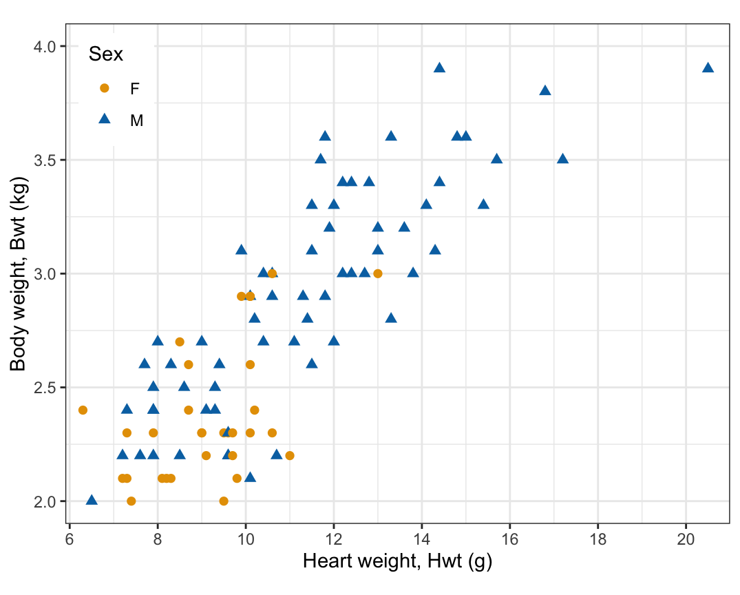
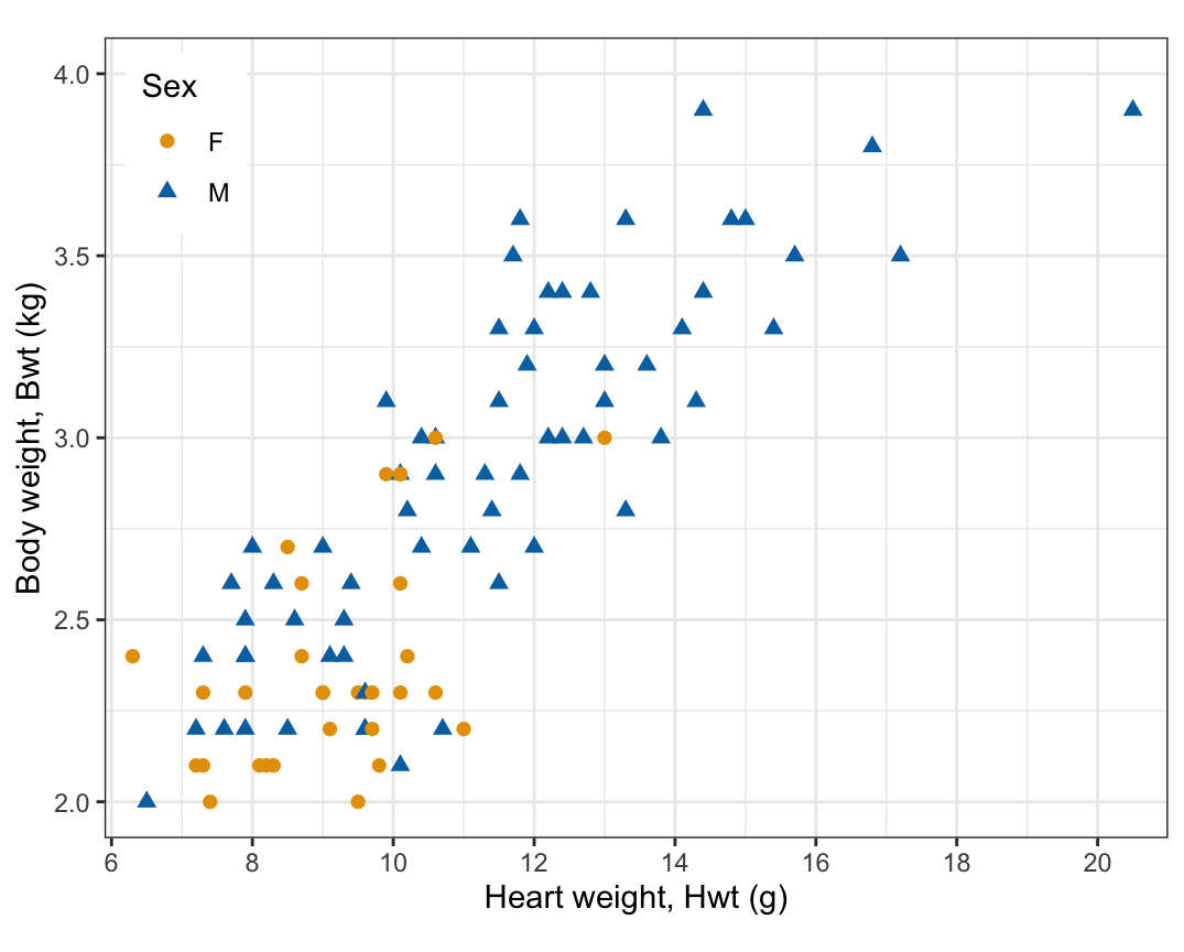
The training cats hold 31 females and 65 males. The males are heavier on average, 2.90 kg against 2.38 kg, with heavier hearts, 11.3 g against 9.2 g, and heart weight rises with body weight in both sexes. Every female weighs at most 3.0 kg, while males run from 2.0 kg up, so the heavier cats are all male and the 71 cats between 2.0 and 3.0 kg are a mixture of the two sexes, with no line between them. The axes are drawn so that one standard deviation of each measurement among the training cats, \(s_{\texttt{Hwt}} = 2.59\) g and \(s_{\texttt{Bwt}} = 0.50\) kg, has the same length; the Standardization section below explains why.
The maximal margin classifier of the previous lecture exists only when a hyperplane separates the classes, and when it exists, one observation near the boundary can move it far. The training cats in the figure above are not separable: in 3 places a female and a male cat share both measurements, and no hyperplane can put one point on both of its sides. The constraints \(y_i\left(\beta_0 + \beta^\top x_i\right) \ge M\) of the maximal margin problem cannot all hold with \(M > 0\).
The support vector classifier (also called the soft margin classifier) allows each observation to violate the margin by an amount it pays for out of a fixed budget. It solves
\[ \begin{aligned} \underset{\beta_0, \beta_1, \ldots, \beta_p, \epsilon_1, \ldots, \epsilon_n, M}{\text{maximize}} \quad & M \\ \text{subject to} \quad & \sum_{j=1}^p \beta_j^2 = 1, \\ & y_i\left(\beta_0 + \beta_1 x_{i1} + \cdots + \beta_p x_{ip}\right) \ge M(1 - \epsilon_i), \\ & \epsilon_i \ge 0, \quad \sum_{i=1}^n \epsilon_i \le C, \end{aligned} \]
where the constraints hold for all \(i = 1, \ldots, n\) and
The pieces:
At the solution, each \(\epsilon_i\) is no larger than its constraint needs, since a smaller \(\epsilon_i\) leaves more of the budget for the others. So \(\epsilon_i\) says where observation \(i\) lies:
Every misclassified training observation uses more than 1 of the budget, so at most \(C\) training observations are misclassified. The cats’ slacks are estimated below, once the classifier is fit.
The support vector classifier of the training cats in the figure above is fit by svm() with kernel = "linear". cost = 1 is a starting value, chosen by cross-validation later. svm() standardizes the features by default, for the reason given in the Standardization section below. As in the previous lecture, tolerance tightens the solver’s stopping rule so that the estimates are accurate to more digits than are printed.
# Support vector classifier: linear kernel, standardized features.
svc_fit <- svm(Sex ~ Hwt + Bwt, data = train, kernel = "linear",
               cost = 1, tolerance = 1e-8)
svc_fit
Call:
svm(formula = Sex ~ Hwt + Bwt, data = train, kernel = "linear", cost = 1,
    tolerance = 1e-08)


Parameters:
   SVM-Type:  C-classification
 SVM-Kernel:  linear
       cost:  1

Number of Support Vectors:  58
The printout gives the settings and the number of support vectors, defined below.
Software solves the problem in a rescaled form, as for the maximal margin classifier. Dividing the second constraint by \(M\) and writing \(w_0 = \beta_0/M\) and \(w = \beta/M\), so that \(\|w\| = 1/M\), it becomes \(y_i\left(w_0 + w^\top x_i\right) \ge 1 - \epsilon_i\), with the same slack \(\epsilon_i\). Maximizing \(M\) is minimizing \(\|w\|\), so the budget problem is
\[ \underset{w_0, w, \epsilon_1, \ldots, \epsilon_n}{\text{minimize}} \quad \tfrac{1}{2}\|w\|^2 \quad \text{subject to} \quad y_i\left(w_0 + w^\top x_i\right) \ge 1 - \epsilon_i, \quad \epsilon_i \ge 0, \quad \sum_{i=1}^n \epsilon_i \le C. \]
e1071::svm() replaces the budget with a price on slack. It solves
\[ \underset{w_0, w, \epsilon_1, \ldots, \epsilon_n}{\text{minimize}} \quad \tfrac{1}{2}\|w\|^2 + \texttt{cost}\sum_{i=1}^n \epsilon_i \quad \text{subject to} \quad y_i\left(w_0 + w^\top x_i\right) \ge 1 - \epsilon_i, \quad \epsilon_i \ge 0, \]
where cost \(> 0\) is its tuning parameter, the price of one unit of slack. (The libsvm documentation behind e1071 writes the slack as \(\xi_i\); it is the same quantity as \(\epsilon_i\).)
cost is not the budget \(C\), and it works in the opposite direction. A large cost makes slack expensive, so the fit buys a narrow margin with few violations, which is a small budget; a small cost makes slack cheap, which is a large budget. The Budget section derives the exact relation.
The margin is a Euclidean distance between points \(x\) and \(x'\), \(\left[\sum_j \left(x_j - x'_j\right)^2\right]^{1/2}\), where \(x_j\) is the \(j\)th coordinate of \(x\) (a single subscript \(j\) on a generic point names a coordinate, and a single subscript \(i\) names an observation). It adds the squared differences of the features in their own units. With heart weight in grams and body weight in kilograms, a difference of 1 g in heart weight counts as much as a difference of 1 kg in body weight, although 1 g is 0.39 standard deviations of heart weight and 1 kg is 1.99 of body weight.
The penalty depends on the units too. Recording feature \(j\) in units \(a\) times smaller multiplies its values by \(a\), so the same hyperplane needs \(w_j/a\) in place of \(w_j\), and its part of \(\|w\|^2\) changes from \(w_j^2\) to \(w_j^2/a^2\). The trade between \(\|w\|^2\) and the slack therefore changes with the units, and the same cost is a different budget.
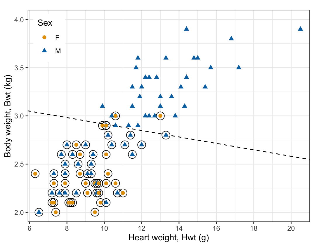
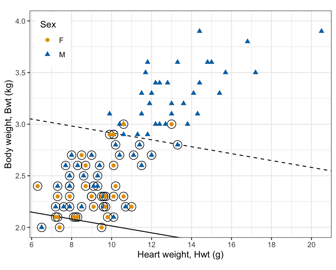
The tabs show two fits with cost = 1: unscaled, with the measurements as recorded (scale = FALSE), and standardized (the fit above). Each has its hyperplane (solid), its margins (dashed), and its support vectors (circled).
# svm()'s rescaled intercept w0 and normal vector w, with M on the positive
# side. svm()'s decision values are positive for the class named first in
# their column name, the class of its first training observation.
svc_w <- function(fit) {
  flip <- if (fit$levels[fit$labels[1]] == "M") 1 else -1
  list(w0 = -flip * fit$rho,
       w = flip * drop(t(fit$coefs) %*% fit$SV))
}

# The same function w0 + w'x written in Hwt (g) and Bwt (kg): undo the
# standardization if svm() used it, and the change to grams if bwt_per_kg
# is 1000.
svc_raw <- function(fit, bwt_per_kg = 1) {
  est <- svc_w(fit)
  center <- c(0, 0)
  spread <- c(1, 1)
  if (!is.null(fit$x.scale)) {
    center <- fit$x.scale[["scaled:center"]]
    spread <- fit$x.scale[["scaled:scale"]]
  }
  slopes <- unname(est$w / spread * c(1, bwt_per_kg))
  c(a0 = est$w0 - sum(est$w * center / spread),
    Hwt = slopes[1],
    Bwt = slopes[2])
}

# The hyperplane (w0 + w'x = 0, solid) and the margins (w0 + w'x = -1 and
# 1, dashed), drawn as lines Bwt = (level - a0 - a1 Hwt) / a2.
svc_lines <- function(a) {
  lapply(c(-1, 0, 1), function(level) {
    geom_abline(intercept = (level - a[["a0"]]) / a[["Bwt"]],
                slope = -a[["Hwt"]] / a[["Bwt"]],
                linetype = if (level == 0) "solid" else "dashed")
  })
}

# A fit drawn over the training cats, with its support vectors circled.
svc_plot <- function(fit, bwt_per_kg = 1, data = train) {
  support <- data[fit$index, ]
  cat_base() +
    svc_lines(svc_raw(fit, bwt_per_kg)) +
    geom_point(data = support, shape = 1, size = 4.5) +
    cat_points()
}
# The same cost unscaled (kg and g as recorded); the standardized fit is
# svc_fit.
fit_raw <- svm(Sex ~ Hwt + Bwt, data = train, kernel = "linear",
cost = 1, scale = FALSE, tolerance = 1e-8)
raw_plot <- svc_plot(fit_raw)
std_plot <- svc_plot(svc_fit)
# Standardized, the fit is the same with body weight in grams.
train_g <- mutate(train, Bwt = 1000 * Bwt)
fit_std_g <- svm(Sex ~ Hwt + Bwt, data = train_g, kernel = "linear",
cost = 1, tolerance = 1e-8)
stopifnot(isTRUE(all.equal(svc_raw(svc_fit),
svc_raw(fit_std_g, bwt_per_kg = 1000),
tolerance = 1e-6)))
# Each fit's w per standard deviation of each measurement: the normal
# vector in the picture, where one standard deviation of each measurement
# is drawn the same length.
per_sd_w <- function(a) {
c(a[["Hwt"]], a[["Bwt"]]) * s_train
}
w_sd_raw <- per_sd_w(svc_raw(fit_raw))
w_sd_std <- per_sd_w(svc_raw(svc_fit))
normal_raw <- w_sd_raw / sqrt(sum(w_sd_raw^2))
normal_std <- w_sd_std / sqrt(sum(w_sd_std^2))
# The angle between the two normal vectors, in degrees.
angle_between <- acos(sum(normal_raw * normal_std)) * 180 / pi
# Margins in the picture (standard deviations): 1 / |w per sd|. The
# standardized one is the margin svm() reports for it; the unscaled fit's
# reported margin, 1 / |w| in kg and g together, is another number.
margin_sd_raw <- 1 / sqrt(sum(w_sd_raw^2))
margin_sd_std <- 1 / sqrt(sum(w_sd_std^2))
w_raw <- svc_w(fit_raw)$w
margin_reported_raw <- 1 / sqrt(sum(w_raw^2))
stopifnot(abs(margin_sd_std - 1 / sqrt(sum(svc_w(svc_fit)$w^2))) < 1e-8)
# The prose reads heart weight's part (first) as positive unscaled and
# negative standardized, and body weight's (second) as positive in both.
stopifnot(normal_raw[1] > 0, normal_std[1] < 0,
normal_raw[2] > 0, normal_std[2] > 0)
# Training error rates and budget used of the two fits.
error_of <- function(fit, data) {
mean(predict(fit, data) != data$Sex)
}
scale_errors <- c(raw = error_of(fit_raw, train),
std = error_of(svc_fit, train))
budget_used <- function(fit, data = train) {
decision <- attr(predict(fit, data, decision.values = TRUE),
"decision.values")
flip <- if (colnames(decision) == "M/F") 1 else -1
sum(pmax(0, 1 - data$y * flip * drop(decision)))
}
scale_budgets <- c(raw = budget_used(fit_raw),
std = budget_used(svc_fit))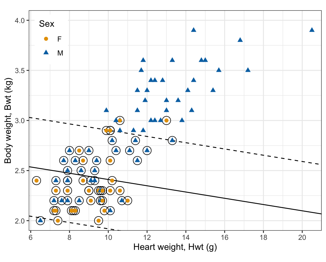
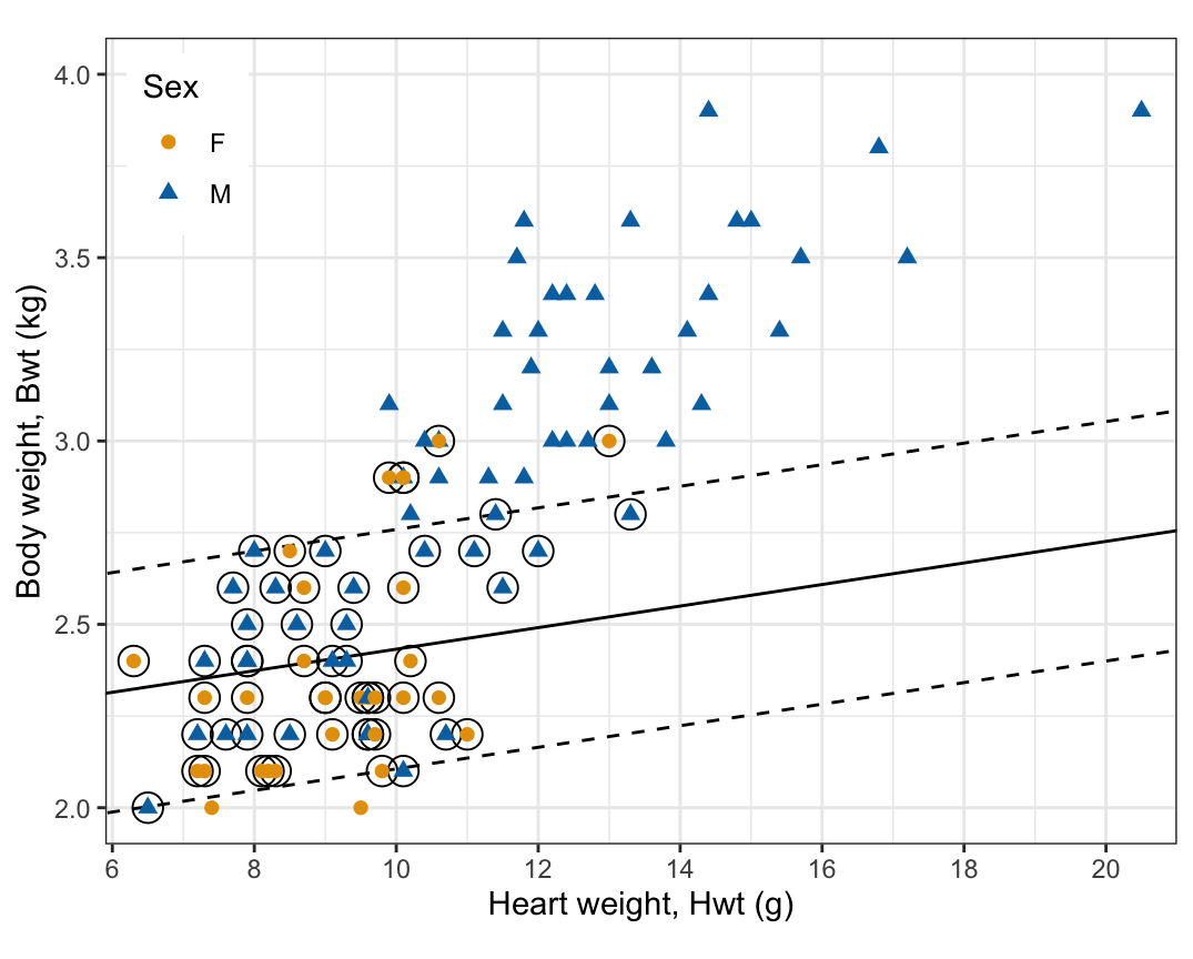
Per standard deviation of each measurement, the unit normal vector of the unscaled fit is \((0.16, 0.99)^\top\) and that of the standardized fit \((-0.15, 0.99)^\top\): both are mostly body weight, and they differ in the sign of the heart weight part, a turn of 17.8 degrees. Their training error rates are 24.0% and 22.9%, and the budgets they use, \(\sum_i\hat\epsilon_i\), are 56.15 and 54.55. The standardized fit’s margins lie \(\hat M = 0.64\) standard deviations from its hyperplane, a distance in the picture. The unscaled fit’s margins lie 0.97 standard deviations from its hyperplane in the picture, but the margin svm() maximizes for it, \(1/\|\hat w\| = 0.49\), is a distance in kilograms and grams together.
Standardizing removes the units. Each feature is replaced by
\[ \tilde x_{ij} = \frac{x_{ij} - \bar x_j}{s_j}, \]
where
sd() computes), andA change of units, \(x_{ij} \to a x_{ij}\) for \(a > 0\), leaves \(\tilde x_{ij}\) unchanged, so the fit no longer depends on the units: refitting the standardized classifier with body weight in grams gives the same hyperplane. svm() does this by default (scale = TRUE): it standardizes each feature with the training observations’ means and standard deviations, stores them in the fit’s x.scale, and applies the same ones to any new observation passed to predict(). The previous lecture set scale = FALSE because both beetle measurements were in micrometers, where a distance in micrometers means something. The cats’ measurements are in different units, so the fits in this lecture standardize.
Undoing the rescaling gives the estimates on the standardized scale,
\[ \hat\beta_0 = \frac{\hat w_0}{\|\hat w\|}, \qquad \hat\beta = \frac{\hat w}{\|\hat w\|}, \qquad \hat M = \frac{1}{\|\hat w\|}, \]
with \(\hat w\) and \(\hat w_0\) read from the fit’s coefs, SV, and rho as in the previous lecture (here SV holds the support vectors’ standardized features). svm()’s decision values are positive for the class of its first training observation, which here is M, so the class coded \(y = 1\).
# w and w0 with M on the positive side.
w_hat <- svc_w(svc_fit)

# Unit-norm estimates on the standardized scale, and the margin.
norm_w <- sqrt(sum(w_hat$w^2))
beta_hat <- c(beta0 = w_hat$w0, w_hat$w) / norm_w
M_hat <- 1 / norm_w
round(c(beta_hat, M = M_hat), 4)
beta0 Hwt Bwt M
0.5519 -0.1502 0.9887 0.6426 # The first training cat is M, and svm()'s decision values, w0 + w'x on the
# standardized scale, are positive for M.
stopifnot(train$Sex[1] == "M")
decision <- attr(predict(svc_fit, train, decision.values = TRUE),
"decision.values")
stopifnot(colnames(decision) == "M/F")
# Standardized features of the training cats, with svm()'s centers and
# scales, which are the training means and standard deviations.
center_train <- svc_fit$x.scale[["scaled:center"]]
scale_train <- svc_fit$x.scale[["scaled:scale"]]
stopifnot(isTRUE(all.equal(scale_train, s_train)))
x_std <- scale(as.matrix(train[c("Hwt", "Bwt")]),
center = center_train, scale = scale_train)
# Fitted values (signed distances in standard deviations), distances on
# each cat's own side, and slacks.
train <- train |>
mutate(f_hat = drop(beta_hat["beta0"] + x_std %*% beta_hat[-1]),
distance = y * f_hat,
slack = pmax(0, 1 - distance / M_hat))
stopifnot(isTRUE(all.equal(drop(decision), train$f_hat * norm_w,
check.attributes = FALSE)))
# The prose reads the average cat as on the M side, heart weight's slope as
# negative and smaller in size, and body weight's as positive (toward M).
stopifnot(beta_hat["beta0"] > 0,
beta_hat["Hwt"] < 0,
beta_hat["Bwt"] > 0,
beta_hat["Bwt"] > abs(beta_hat["Hwt"]))The fitted value \(\hat f(x) = \hat\beta_0 + \hat\beta_1\tilde x_1 +
\hat\beta_2\tilde x_2\) is the signed distance from \(x\) to the hyperplane in the standardized features, in standard deviations, with \(\tilde x_1\) and \(\tilde x_2\) the standardized heart and body weights. \(\hat\beta_0 = 0.55\) is \(\hat f\) at \(\tilde x = 0\), a cat of average heart and body weight among the training cats: it lies 0.55 standard deviations from the hyperplane on the M side. \(\hat\beta_1 = -0.15\): one standard deviation more heart weight (2.59 g) moves a cat 0.15 standard deviations toward the F side. \(\hat\beta_2 = 0.99\): one standard deviation more body weight (0.50 kg) moves it 0.99 standard deviations toward the M side. Body weight carries most of the classification; among cats of the same body weight, a heavier heart points slightly toward female. The margin is \(\hat M = 0.64\) standard deviations.
Each \(\hat\epsilon_i\) is the smallest slack its constraint allows,
\[ \hat\epsilon_i = \max\left(0,\ 1 - \frac{y_i \hat f(x_i)}{\hat M}\right), \]
where \(y_i \hat f(x_i)/\hat M\) is observation \(i\)’s distance from the hyperplane on its own side, in margins. The first tab is the fit; the second plots each training cat’s \(\hat\epsilon_i\) against \(y_i\hat f(x_i)/\hat M\), with the three kinds of observation shaded.
# The three kinds of training cat, by slack, up to the solver's accuracy
# (1e-4, as for the plateau below).
kinds <- c("On or outside the margin", "Inside the margin", "Wrong side")
train <- train |>
  mutate(kind = case_when(slack < 1e-4 ~ kinds[1],
                          slack <= 1 ~ kinds[2],
                          TRUE ~ kinds[3]),
         kind = factor(kind, levels = kinds))
kind_counts <- table(train$kind)

# Training cats on the margin: slack 0, at distance M_hat.
n_on_margin <- sum(abs(train$distance / M_hat - 1) < 1e-4)

# The estimated budget used, the sum of the slacks.
C_hat <- sum(train$slack)

fit_plot <- svc_plot(svc_fit)

# Shaded bands for the three kinds, and the hinge max(0, 1 - u).
u_limits <- c(-3.5, 4.5)
bands <- tibble(xmin = c(1, 0, u_limits[1]),
                xmax = c(u_limits[2], 1, 0),
                kind = factor(kinds, levels = kinds))
hinge <- tibble(u = c(u_limits[1], 1, u_limits[2])) |>
  mutate(slack = pmax(0, 1 - u))
stopifnot(between(range(train$distance / M_hat),
                  u_limits[1], u_limits[2]))

slack_plot <- ggplot(train, aes(x = distance / M_hat, y = slack)) +
  geom_rect(data = bands,
            aes(xmin = xmin, xmax = xmax, ymin = -Inf, ymax = Inf,
                fill = kind),
            inherit.aes = FALSE) +
  geom_line(data = hinge, aes(x = u, y = slack), color = "grey50") +
  geom_point(aes(color = Sex, shape = Sex), size = 2) +
  annotate("text", x = c(2.75, 0.5, -1.75), y = 4.25,
           label = c("On or outside\nthe margin", "Inside the\nmargin",
                     "Wrong side")) +
  scale_fill_manual(values = c("white", "grey92", "grey80"),
                    guide = "none") +
  scale_color_manual(values = sex_colors) +
  scale_shape_manual(values = sex_shapes) +
  scale_x_continuous(breaks = seq(-3, 4, by = 1),
                     minor_breaks = seq(-3.5, 4.5, by = 1)) +
  scale_y_continuous(breaks = seq(0, 4, by = 1),
                     minor_breaks = seq(0.5, 4.5, by = 1)) +
  coord_cartesian(xlim = u_limits, ylim = c(-0.2, 4.8), expand = FALSE) +
  labs(x = expression("Distance on own side, in margins, " *
                        y[i] * hat(f)(x[i]) / hat(M)),
       y = expression("Slack, " * hat(epsilon)[i]),
       color = "Sex", shape = "Sex") +
  theme(legend.position = "inside",
        legend.position.inside = c(0.98, 0.6),
        legend.justification = c(1, 1))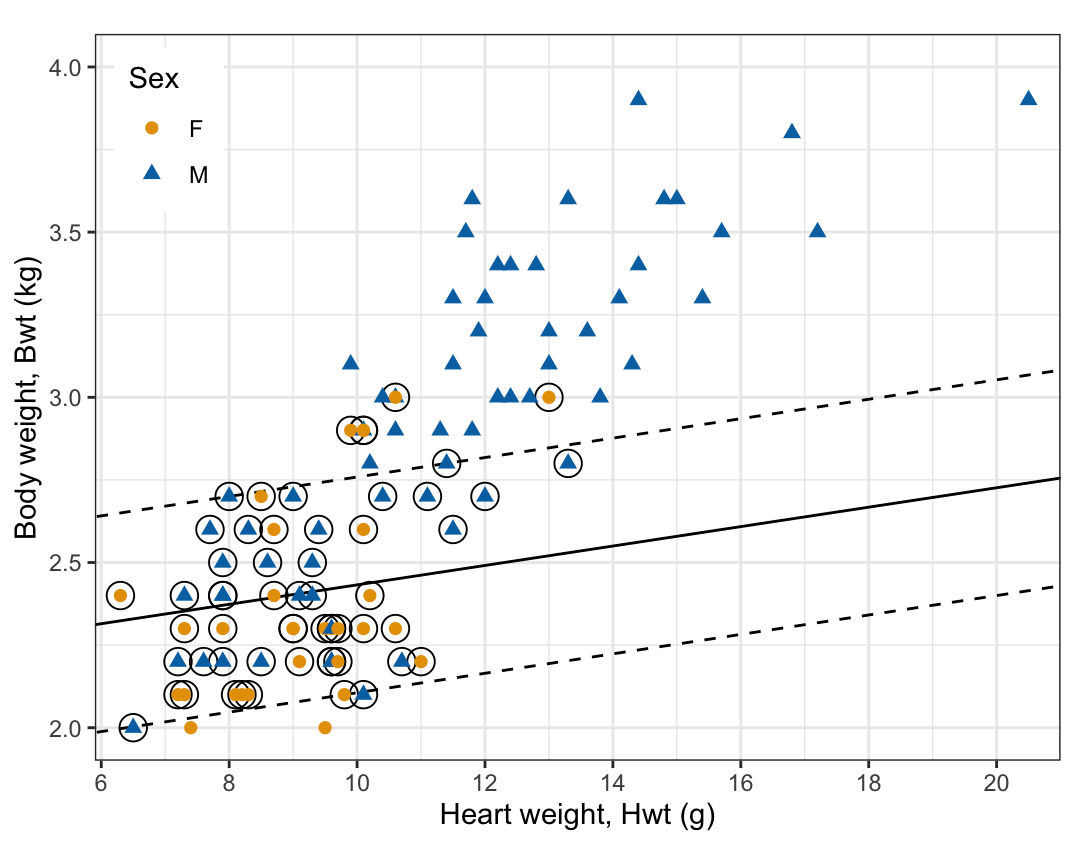
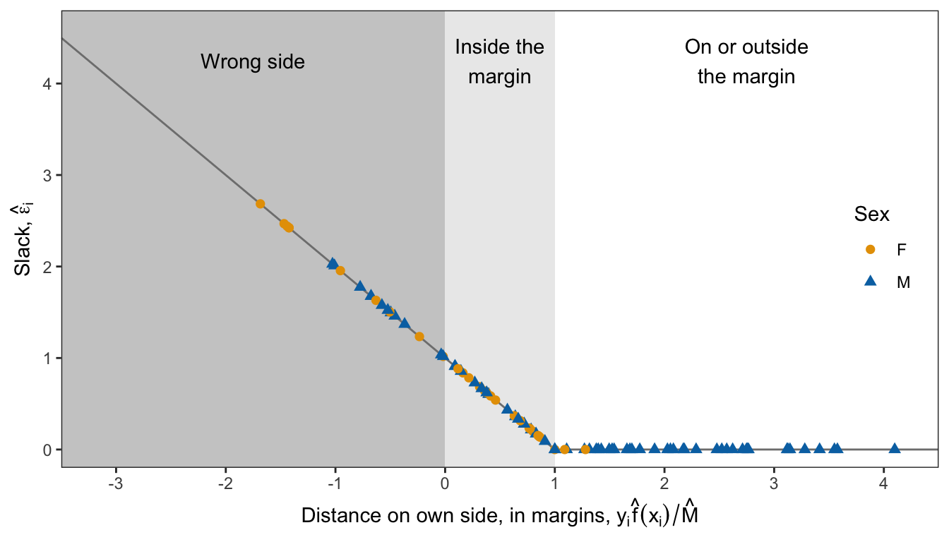
Of the 96 training cats, 41 are on or outside the margin (3 of them exactly on it) with \(\hat\epsilon_i = 0\), 33 are inside the margin on the correct side, and 22 are on the wrong side of the hyperplane, so the training error rate is 22.9%. The slacks lie on the line \(\hat\epsilon_i = 1 - y_i\hat f(x_i)/\hat M\) to the left of 1 and at 0 to its right. They add to \(\sum_i\hat\epsilon_i = 54.55\), the budget this fit uses. The misclassified cats are the lighter males, below the solid line, and the heavier females, above it.
The tabs show the training cats and then support vector classifiers fit with four values of cost, from small to large, each with its hyperplane, margins, and support vectors circled.
# Fits at four values of cost.
tab_costs <- c(0.01, 0.1, 1, 10)
tab_fits <- lapply(tab_costs, function(cost) {
  svm(Sex ~ Hwt + Bwt, data = train, kernel = "linear",
      cost = cost, tolerance = 1e-8)
})
tab_plots <- lapply(tab_fits, svc_plot)

# Margin, budget used, and kinds of training cat of a fit.
svc_summary <- function(fit, data = train) {
  est <- svc_w(fit)
  decision <- attr(predict(fit, data, decision.values = TRUE),
                   "decision.values")
  flip <- if (colnames(decision) == "M/F") 1 else -1
  margins_out <- data$y * flip * drop(decision)
  slack <- pmax(0, 1 - margins_out)
  tibble(cost = fit$cost,
         C = sum(slack),
         M = 1 / sqrt(sum(est$w^2)),
         n_support = fit$tot.nSV,
         n_inside = sum(slack > 1e-4 & slack <= 1),
         n_wrong = sum(slack > 1),
         error = mean(predict(fit, data) != data$Sex))
}
budget_summary <- map_dfr(tab_fits, svc_summary)

# The budget used falls, and the margin narrows, as cost grows.
stopifnot(!is.unsorted(rev(budget_summary$C)),
          !is.unsorted(rev(budget_summary$M)))

# At the smallest cost every training cat is classified M, so every
# female is on the wrong side.
smallest <- budget_summary[1, ]
stopifnot(all(predict(tab_fits[[1]], train) == "M"),
          smallest$n_wrong == sum(train$Sex == "F"))

budget_table <- budget_summary |>
  knitr::kable(digits = c(2, 2, 2, 0, 0, 0, 3),
               col.names = c("`cost`", "$\\sum_i\\hat\\epsilon_i$",
                             "$\\hat M$", "Support vectors",
                             "Inside the margin", "Wrong side",
                             "Training error rate"),
               align = "rrrrrrr")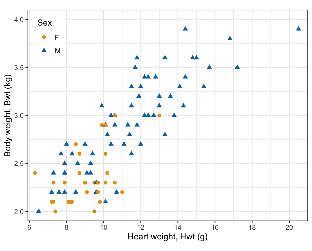
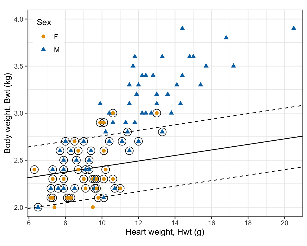
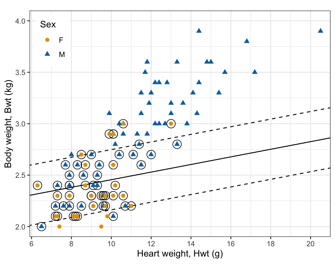
The budget \(C\) is the classifier’s tuning parameter.
With cost = 0.01 slack is so cheap that the margin is 17.7 standard deviations. The hyperplane and the margin on the F side lie off the plot below; only the margin on the M side (dashed) is in view. Every training cat is classified M, the more common sex, so every female is on the wrong side, and the 62 support vectors are the 31 females and the 31 males below the dashed line. As cost grows the margin narrows and the hyperplane turns to separate light from heavy cats, but it changes little from cost = 1 to 10.
svm()’s penalty form solves the budget problem, for a budget set by cost. Let \((\hat w_0, \hat w, \hat\epsilon)\) solve the penalty problem at some cost, and let \(C = \sum_i\hat\epsilon_i\). Any \((w_0, w, \epsilon)\) that satisfies the budget problem’s constraints with this \(C\) also satisfies the penalty problem’s, so
\[ \tfrac12\|w\|^2 + \texttt{cost}\sum_i\epsilon_i \ \ge\ \tfrac12\|\hat w\|^2 + \texttt{cost}\, C, \quad\text{so}\quad \tfrac12\|w\|^2 \ \ge\ \tfrac12\|\hat w\|^2 + \texttt{cost}\left(C - \sum_i\epsilon_i\right) \ \ge\ \tfrac12\|\hat w\|^2, \]
because \(\sum_i\epsilon_i \le C\). No point within the budget has a smaller \(\|w\|\), so \(\hat w\) solves the budget problem with budget \(C = \sum_i\hat\epsilon_i\).
The budget does not grow as cost grows. Write \(N = \tfrac12\|\hat w\|^2\) and \(S = \sum_i\hat\epsilon_i\) for the solution at cost \(= a\), and \(N'\) and \(S'\) for the solution at cost \(= b > a\). Each solution is at least as good as the other at its own cost:
\[ N + aS \le N' + aS', \qquad N' + bS' \le N + bS. \]
Adding the two gives \(aS + bS' \le aS' + bS\), that is, \((b - a)(S' - S) \le 0\), so \(S' \le S\): the larger cost uses no more budget. Then the first inequality gives \(N \le N'\): the larger cost has a margin \(1/\|\hat w\|\) no wider. So the budget is a weakly monotone function of cost, a larger cost corresponding to a budget no larger, and it can be constant on a plateau (the cats have one, shown in the Support vectors section). cost and \(C\) are not equal, and the \(C\) that a cost gives depends on the data. As cost grows without bound on separable data, the budget falls to 0 and the fit becomes the maximal margin classifier, which is why the previous lecture used a very large cost. For the four fits in the tabs:
cost |
\(\sum_i\hat\epsilon_i\) | \(\hat M\) | Support vectors | Inside the margin | Wrong side | Training error rate |
|---|---|---|---|---|---|---|
| 0.01 | 61.68 | 17.68 | 62 | 31 | 31 | 0.323 |
| 0.10 | 58.80 | 1.77 | 62 | 34 | 28 | 0.292 |
| 1.00 | 54.55 | 0.64 | 58 | 33 | 22 | 0.229 |
| 10.00 | 54.41 | 0.57 | 56 | 32 | 21 | 0.219 |
The budget used, \(\sum_i\hat\epsilon_i\), and the margin \(\hat M\) fall as cost grows. The budget stays above the number of misclassified training cats, as it must.
The figure is the fit with cost = 1 again.
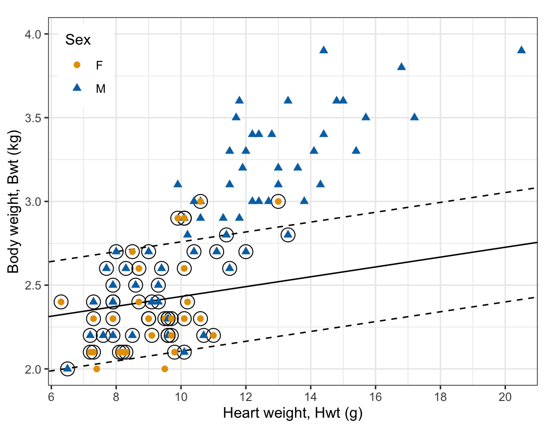
The support vectors of the support vector classifier are the training observations on the margin, inside it, or on the wrong side of the hyperplane: those with \(y_i\hat f(x_i) \le \hat M\). This is wider than the previous lecture’s definition, the observations on the margin only, which is the case with no slack. They are the circled cats, 58 of the 96: the 3 on the margin, with \(\hat\epsilon_i = 0\), and all 55 with \(\hat\epsilon_i > 0\).
# Training cats on or inside the margin or on the wrong side.
support <- filter(train, distance / M_hat < 1 + 1e-4)
count(support, kind)
kind n
1 On or outside the margin 3
2 Inside the margin 33
3 Wrong side 22# The cats with distance at most M_hat are the rows svm() kept.
stopifnot(setequal(which(train$distance / M_hat < 1 + 1e-4),
svc_fit$index))
# Support vectors: on the margin, or with positive slack.
stopifnot(svc_fit$tot.nSV == n_on_margin + sum(train$slack > 1e-4))
# Refits on standardized features, with the training cats' means and
# standard deviations: all training cats, and the support vectors alone.
train_std <- tibble(Sex = train$Sex,
Hwt = x_std[, "Hwt"],
Bwt = x_std[, "Bwt"])
refit_std <- function(data) {
fit <- svm(Sex ~ Hwt + Bwt, data = data, kernel = "linear",
cost = 1, scale = FALSE, tolerance = 1e-8)
w <- svc_w(fit)
c(w$w0, w$w) / sqrt(sum(w$w^2))
}
beta_all <- refit_std(train_std)
beta_support <- refit_std(train_std[svc_fit$index, ])
# Both agree with the standardized fit to six decimal places.
stopifnot(max(abs(beta_all - beta_hat)) < 1e-6,
max(abs(beta_support - beta_hat)) < 1e-6)The fitted hyperplane depends on the training data only through the support vectors. An observation outside the margin has \(\hat\epsilon_i = 0\) and its constraint holds with room to spare. Suppose deleting it allowed a better solution. Moving from the current solution a short way toward that better one keeps the deleted observation’s constraint satisfied (it held strictly), keeps every other constraint satisfied (each defines a convex set that contains both ends), and lowers the objective (which is convex). That point would then beat the current solution of the full problem, which is impossible. So deleting an observation outside the margin, or moving it anywhere outside the margin, leaves the fit unchanged. Refitting the standardized problem to the 58 support vectors alone, with the training cats’ means and standard deviations, gives the same estimates to six decimal places.
The difference from the maximal margin classifier is how many support vectors there are. There, a handful of observations on the margin set the hyperplane; here every observation inside the margin or on the wrong side does, and a wider margin holds more of them.
The figure counts the support vectors, and the two kinds with positive slack, for fits over a grid of cost values.
# Fits over a grid of cost, 4 per factor of 10.
cost_grid <- 10^seq(-2, 2, by = 0.25)
grid_summary <- map_dfr(cost_grid, function(cost) {
  fit <- svm(Sex ~ Hwt + Bwt, data = train, kernel = "linear",
             cost = cost, tolerance = 1e-8)
  svc_summary(fit)
})

# Counts by kind, long, for one line per kind.
count_levels <- c("Support vectors", "Inside the margin", "Wrong side")
count_long <- grid_summary |>
  select(cost, n_support, n_inside, n_wrong) |>
  pivot_longer(-cost, names_to = "what", values_to = "count") |>
  mutate(what = factor(what,
                       levels = c("n_support", "n_inside", "n_wrong"),
                       labels = count_levels))

# Log axis for cost: majors at powers of 10, minors midway in log space.
cost_axis <- scale_x_log10(breaks = 10^(-2:2),
                           minor_breaks = 10^seq(-1.5, 1.5, by = 1),
                           labels = c("0.01", "0.1", "1", "10", "100"))

count_plot <- ggplot(count_long,
                     aes(x = cost, y = count,
                         color = what, shape = what, linetype = what)) +
  geom_line() +
  geom_point(size = 2) +
  cost_axis +
  scale_y_continuous(breaks = seq(0, 70, by = 10),
                     minor_breaks = seq(5, 65, by = 10)) +
  scale_color_manual(values = c("black", "#009E73", "#CC79A7")) +
  coord_cartesian(xlim = c(0.008, 125), ylim = c(0, 70), expand = FALSE) +
  labs(x = "cost (log scale)", y = "Training cats",
       color = NULL, shape = NULL, linetype = NULL) +
  theme(legend.position = "inside",
        legend.position.inside = c(0.98, 0.03),
        legend.justification = c(1, 0))

grid_first <- grid_summary[1, ]
grid_last <- grid_summary[nrow(grid_summary), ]
# The budget used never rises with cost (up to the solver's accuracy), and
# from some cost on the fit stops changing.
stopifnot(all(diff(grid_summary$C) < 1e-4),
          all(grid_summary$n_support > nrow(train) / 2),
          min(grid_summary$n_wrong) == grid_last$n_wrong)
plateau <- grid_summary |>
  filter(abs(C - grid_last$C) < 1e-4, abs(M - grid_last$M) < 1e-4)
plateau_cost <- min(plateau$cost)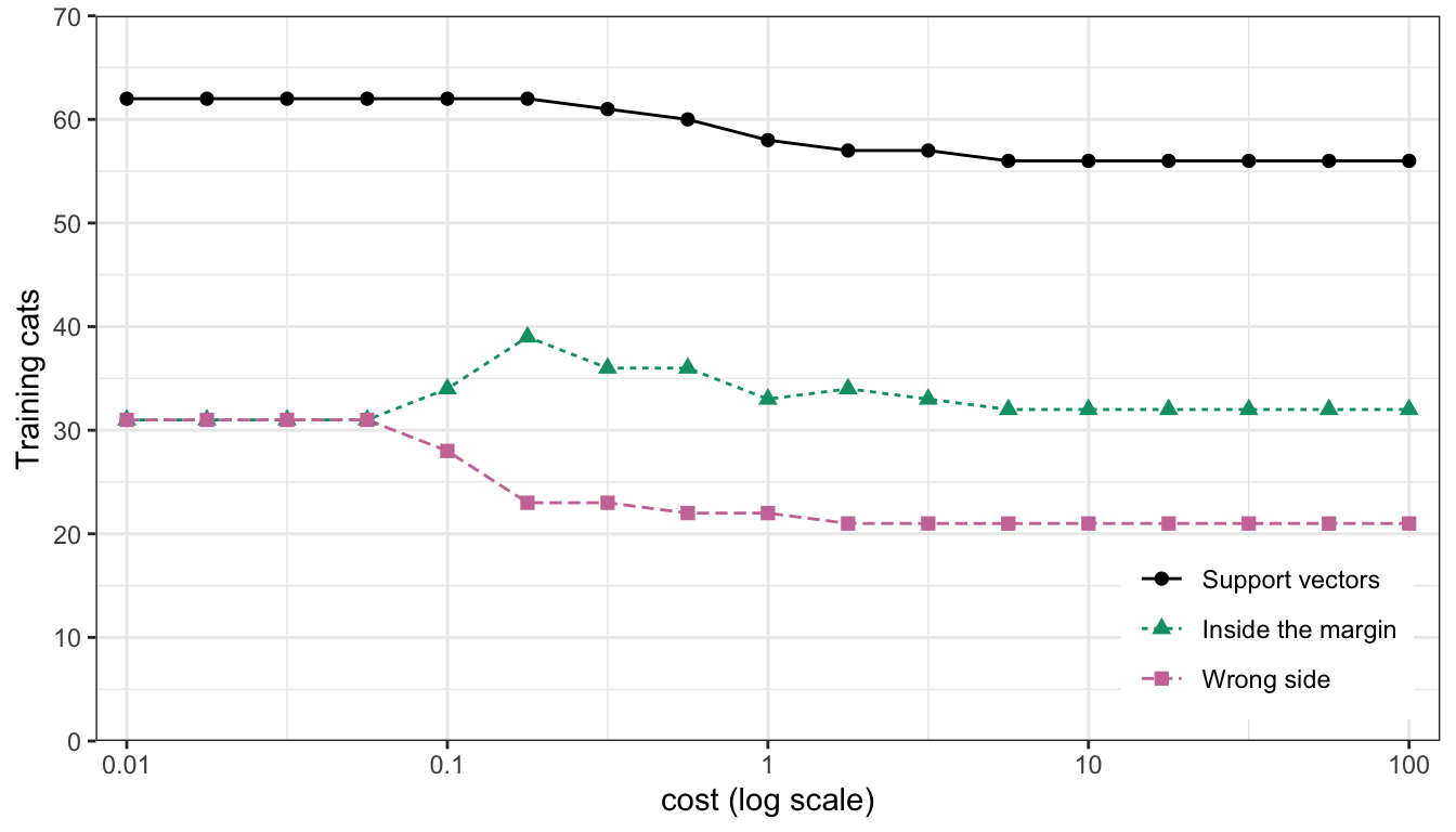
The number of support vectors falls from 62 at cost = 0.01 to 56 at cost = 100, as the margin narrows from 17.7 to 0.57 standard deviations. Because the sexes overlap so much, more than half of the training cats are support vectors at every cost, including the 21 or more misclassified training cats of every fit on the grid. From cost = 5.62 on, the fit no longer changes: its budget used, 54.41, is the smallest total slack that any hyperplane leaves these training cats, so a larger cost cannot reduce it.
The figure is the training cats from the start of the lecture. Cross-validation chooses cost from them alone; the test cats stay aside.
The budget, and so cost, is chosen by cross-validation, as in the resampling lectures. With the training cats split at random into \(k = 10\) folds \(\mathcal{F}_1, \ldots, \mathcal{F}_{10}\) of sizes \(n_\ell\), the estimate for a given cost is
\[ \text{CV}_{(10)}(\texttt{cost}) = \frac{1}{10}\sum_{\ell=1}^{10}\text{Err}_\ell, \qquad \text{Err}_\ell = \frac{1}{n_\ell}\sum_{i \in \mathcal{F}_\ell} \mathrm{I}\left(y_i \ne \hat y_i^{(-\ell)}\right), \]
where \(\hat y_i^{(-\ell)}\) is the class predicted for observation \(i\) by the support vector classifier fit with that cost to the training cats outside fold \(\ell\), and \(\text{Err}_\ell\) is its error rate on fold \(\ell\). e1071::tune() averages the fold error rates with equal weights, so with folds of different sizes it differs slightly from the size-weighted average of the resampling lectures. Each fit inside tune() standardizes with its own training folds’ means and standard deviations, so the standardization is part of the fit being cross-validated.
tune() takes the fitting function, the model, any further arguments for it, and a list of values of the tuning parameter. Its folds are random, which the seed set at the top of this file makes reproducible. The fits inside it keep svm()’s default tolerance; with the tighter one, the solver stops at its iteration limit on some folds.
# 10-fold cross-validation over the grid of cost values.
cv_fit <- tune(svm, Sex ~ Hwt + Bwt, data = train, kernel = "linear",
               ranges = list(cost = cost_grid))
head(cv_fit$performances, 3)
cost error dispersion
1 0.01000000 0.3255556 0.1478747
2 0.01778279 0.3255556 0.1478747
3 0.03162278 0.3255556 0.1478747cv_fit$best.parameters cost
10 1.778279The performances table has one row per cost: error is \(\text{CV}_{(10)}(\texttt{cost})\), by default the misclassification rate, and dispersion the standard deviation of the 10 fold error rates. best.parameters is the cost with the smallest error (the smallest such cost if several tie), and best.model is the support vector classifier refit with it to all the training cats.
# The cross-validation estimate against cost, and the chosen cost.
cv_table <- as_tibble(cv_fit$performances)
best_cost <- cv_fit$best.parameters$cost
best_row <- filter(cv_table, cost == best_cost)

# Error rate of classifying every training cat M.
all_M_error <- mean(train$Sex != "M")

cv_plot <- ggplot(cv_table, aes(x = cost, y = error)) +
  geom_hline(yintercept = all_M_error, linetype = "dotted") +
  annotate("text", x = 20, y = all_M_error + 0.02,
           label = "Every cat classified M") +
  geom_line() +
  geom_point(size = 2) +
  geom_point(data = best_row, shape = 1, size = 5) +
  cost_axis +
  scale_y_continuous(breaks = seq(0, 0.4, by = 0.1),
                     minor_breaks = seq(0.05, 0.45, by = 0.1),
                     labels = scales::label_percent()) +
  coord_cartesian(xlim = c(0.008, 125), ylim = c(0, 0.42),
                  expand = FALSE) +
  labs(x = "cost (log scale)",
       y = "10-fold CV estimate of error rate")

# The smallest costs' estimates are close to the all-M error rate.
stopifnot(abs(cv_table$error[1] - all_M_error) < 0.01)

# Training error rate of the chosen fit.
svc_best <- cv_fit$best.model
best_train_error <- error_of(svc_best, train)
stopifnot(svc_best$cost == best_cost)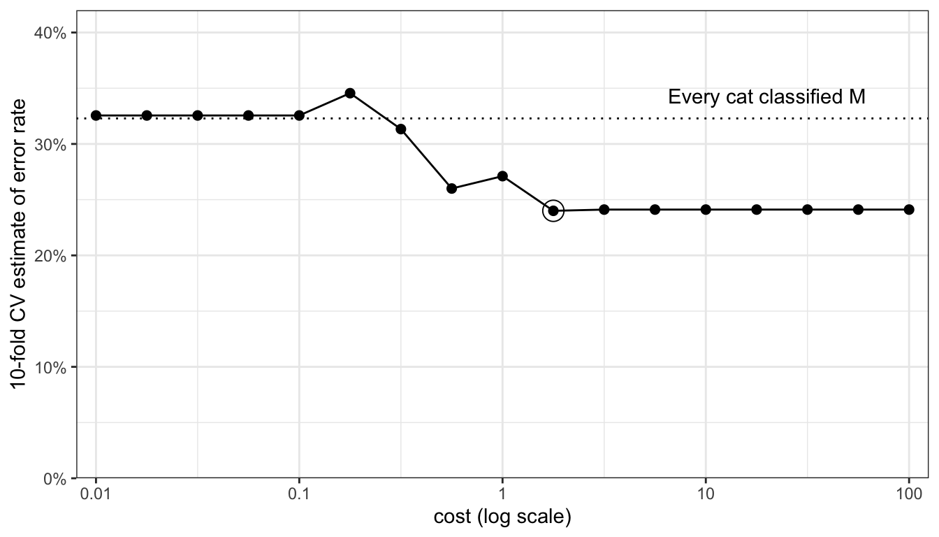
For small cost, the estimate is close to the error rate of classifying every training cat M (dotted): the margin is so wide that the classifier fit to each set of training folds puts nearly every cat on the M side. The estimate is not monotone in cost (it rises to 34.6% at cost = 0.18); it is smallest, 24.0%, at cost = 1.78 (circled), after which it is nearly flat. A linear boundary in two features has only three estimates, so even the narrowest margin on this grid varies little from one set of training folds to another, and the curve does not rise again at large cost. The fold error rates at the chosen cost have standard deviation 16.0%, so differences of a few percentage points along the curve are within the noise of the estimate.
The figure shows the 48 test cats and the support vector classifier chosen by cross-validation, refit to all the training cats, with its hyperplane and margins; crosses mark the test cats it misclassifies.
# Test cats, their fitted values, and the misclassified ones.
test <- test |>
  mutate(predicted = predict(svc_best, test))
wrong_test <- filter(test, predicted != Sex)

test_plot <- cat_base() +
  svc_lines(svc_raw(svc_best)) +
  cat_points(test) +
  geom_point(data = wrong_test, shape = 4, size = 3.5, stroke = 1)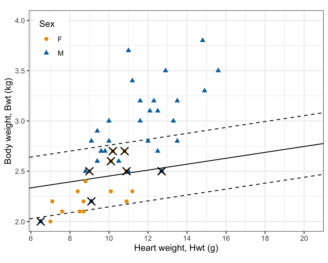
A new observation \(x^*\) is classified by the sign of \(\hat f(x^*)\), as for the maximal margin classifier: to M if \(\hat f(x^*) > 0\) and to F if \(\hat f(x^*) < 0\). predict() standardizes \(x^*\) with the training cats’ means and standard deviations first.
# Predicted sex of the first test cats.
head(select(test, Sex, Hwt, Bwt, predicted))
Sex Hwt Bwt predicted
1 F 7.0 2.0 F
6 F 7.6 2.1 F
10 F 8.5 2.1 F
11 F 8.7 2.1 F
13 F 7.1 2.2 F
14 F 8.7 2.2 FWith M, the class coded \(y = 1\), as the positive class, the confusion matrix of the test cats is
# Truth in the rows, predictions in the columns.
confusion <- table(Truth = test$Sex, Predicted = test$predicted)
confusion
Predicted
Truth F M
F 11 5
M 4 28The test error rate is \((FP + FN)/n = (5 + 4)/48 =
0.188\), against 33.3% for classifying every test cat M. The sensitivity, the proportion of male cats classified male, is 87.5%, and the specificity, the proportion of female cats classified female, is 68.8%. The training error rate of the same fit is 21.9% and its cross-validation estimate 24.0%; the test cats played no part in fitting or in choosing cost, so the test error rate is the honest estimate, if a noisy one from 48 cats. The misclassified test cats lie where the training cats of the two sexes overlapped: the lighter males and the heavier females.
The penalty form can be rewritten without the slack variables as minimizing \(\sum_i \max\left[0,\ 1 - y_i\left(w_0 + w^\top x_i\right)\right] +
\tfrac{1}{2\,
\texttt{cost}}\|w\|^2\), a loss plus a ridge-like penalty; the next lecture compares this loss with logistic regression’s. svm() has other options not taught here: class.weights sets a different cost for each class, which matters when one class is rare or its errors are costlier; type = "nu-classification" replaces cost with a parameter \(\nu\) that is a lower bound on the fraction of support vectors and an upper bound on the fraction of observations inside the margin or on the wrong side; and type = "one-classification" fits a one-class support vector machine, which describes where a single class lies in order to flag unusual new observations. In the Lagrangian dual of the penalty form, each observation’s multiplier is bounded above by cost. See The Elements of Statistical Learning (Hastie, Tibshirani, and Friedman), Section 12.2.
The comparison classifiers come from the earlier lectures. Each is fit to the same 96 training cats and the same two explanatory variables, Hwt and Bwt, gives a probability that a cat is M, and classifies it M when that probability exceeds \(1/2\):
Hwt and Bwt, and with both squares as well as the interaction;randomForest()’s default settings.The support vector classifier is the one chosen by cross-validation in this lecture, with cost = 1.78. The calls for main-effects logistic regression, LDA, QDA and the random forest, and the probabilities LDA gives the first three test cats, are
# Fits to the training cats; each gives a probability that a cat is M.
set.seed(20261114)
logit_fit <- glm(Sex ~ Hwt + Bwt, data = train, family = binomial)
lda_fit <- MASS::lda(Sex ~ Hwt + Bwt, data = train)
qda_fit <- MASS::qda(Sex ~ Hwt + Bwt, data = train)
rf_fit <- randomForest::randomForest(Sex ~ Hwt + Bwt, data = train)

# Probabilities of F and M that LDA gives the first three test cats.
head(predict(lda_fit, test)$posterior, 3)
F M
1 0.7219232 0.2780768
6 0.6667787 0.3332213
10 0.6774822 0.3225178# Ten folds of the training cats, the same for every classifier.
set.seed(20261114)
fold <- sample(rep(1:10, length.out = nrow(train)))
# Probability of M from each kind of fit.
glm_prob <- function(model, data) {
predict(model, data, type = "response")
}
posterior_prob <- function(model, data) {
predict(model, data)$posterior[, "M"]
}
forest_prob <- function(model, data) {
predict(model, data, type = "prob")[, "M"]
}
# Each classifier: how to fit it to a data set, and its probability of M.
logit_inter <- Sex ~ Hwt * Bwt
logit_quad <- Sex ~ Hwt + Bwt + I(Hwt^2) + I(Bwt^2) + Hwt:Bwt
classifiers <- list(
"Logistic, main effects" = list(
fit = function(data) {
glm(Sex ~ Hwt + Bwt, data = data, family = binomial)
},
prob = glm_prob),
"Logistic, interaction" = list(
fit = function(data) {
glm(logit_inter, data = data, family = binomial)
},
prob = glm_prob),
"Logistic, quadratic" = list(
fit = function(data) {
glm(logit_quad, data = data, family = binomial)
},
prob = glm_prob),
"LDA" = list(
fit = function(data) {
MASS::lda(Sex ~ Hwt + Bwt, data = data)
},
prob = posterior_prob),
"QDA" = list(
fit = function(data) {
MASS::qda(Sex ~ Hwt + Bwt, data = data)
},
prob = posterior_prob),
"Random forest" = list(
fit = function(data) {
randomForest::randomForest(Sex ~ Hwt + Bwt, data = data)
},
prob = forest_prob))
# Test probabilities: the fits above, and the other two logistic regressions
# fit to all the training cats.
test_fits <- list(
"Logistic, main effects" = logit_fit,
"Logistic, interaction" = classifiers[[2]]$fit(train),
"Logistic, quadratic" = classifiers[[3]]$fit(train),
"LDA" = lda_fit,
"QDA" = qda_fit,
"Random forest" = rf_fit)
test_prob <- map2(classifiers, test_fits, function(classifier, model) {
classifier$prob(model, test)
})
# Cross-validation probabilities: each training cat's probability from a fit
# to the other nine folds.
cv_prob <- map(classifiers, function(classifier) {
prob <- numeric(nrow(train))
for (k in 1:10) {
inside <- fold != k
model <- classifier$fit(train[inside, ])
prob[!inside] <- classifier$prob(model, train[!inside, ])
}
prob
})
# The support vector classifier gives classes only. It is refit in each fold
# at the cost chosen above, with tune()'s default tolerance.
cv_class <- character(nrow(train))
for (k in 1:10) {
inside <- fold != k
model <- svm(Sex ~ Hwt + Bwt, data = train[inside, ], kernel = "linear",
cost = svc_best$cost)
cv_class[!inside] <- as.character(predict(model, train[!inside, ]))
}
# Error rate of probabilities classified at 1/2, and log loss: minus the
# mean log of the probability given each cat's observed sex.
error_rate <- function(p, sex) {
mean((p > 0.5) != (sex == "M"))
}
log_loss <- function(p, sex) {
-mean(ifelse(sex == "M", log(p), log(1 - p)))
}
# The comparison, one row per classifier, the support vector classifier last.
# It has no probabilities, so no log loss.
comparison <- tibble(
classifier = c(names(classifiers), "Support vector classifier"),
test_error = c(sapply(test_prob, error_rate, sex = test$Sex),
mean(test$predicted != test$Sex)),
cv_error = c(sapply(cv_prob, error_rate, sex = train$Sex),
mean(cv_class != train$Sex)),
test_loss = c(sapply(test_prob, log_loss, sex = test$Sex), NA),
cv_loss = c(sapply(cv_prob, log_loss, sex = train$Sex), NA))
# A random forest's vote fractions can be exactly 0 or 1, which would make
# its log loss infinite; they are not here. (The quadratic logistic regression
# warns that fitted probabilities are numerically 0 or 1 in one fold; its log
# loss is finite.)
stopifnot(all(is.finite(comparison$test_loss[1:6])),
all(is.finite(comparison$cv_loss[1:6])))
stopifnot(comparison$test_error[7] == test_error)
# Facts the prose reads off the table.
others <- comparison[1:6, ]
svc_row <- comparison[7, ]
main_row <- comparison[1, ]
flexible <- others[c(2, 3, 5, 6), ]
stopifnot(!any(flexible$test_error < main_row$test_error &
flexible$cv_error < main_row$cv_error))
flex_names <- c("Logistic, quadratic", "QDA", "Random forest")
low_test_loss <- others$classifier[rank(others$test_loss) <= 3]
high_cv_loss <- others$classifier[rank(others$cv_loss) >= 4]
stopifnot(setequal(low_test_loss, flex_names),
setequal(high_cv_loss, flex_names))
# Test cats each classifier misclassifies, and the support vector
# classifier's difference from them.
missed <- round(comparison$test_error * nrow(test))
svc_vs <- missed[7] - missed[1:6]
stopifnot(all(svc_vs[1:4] == 1),
which.min(others$test_error) == 5,
which.max(others$cv_error) == 5)
# Log loss of giving every cat the proportion of males among the training
# cats, and in cross-validation among the cats outside its fold.
p_constant <- mean(train$Sex == "M")
test_loss_constant <- log_loss(rep(p_constant, nrow(test)), test$Sex)
p_cv_constant <- numeric(nrow(train))
for (k in 1:10) {
inside <- fold != k
p_cv_constant[!inside] <- mean(train$Sex[inside] == "M")
}
cv_loss_constant <- log_loss(p_cv_constant, train$Sex)
# One table: all the cross-validation columns first, then all the test
# columns. Error rates in percent; the support vector classifier has no
# log loss, shown as a dash.
options(knitr.kable.NA = "—")
comparison_table <- comparison |>
transmute(classifier,
cv_error = 100 * cv_error,
cv_loss,
test_error = 100 * test_error,
test_loss) |>
knitr::kable(digits = c(0, 1, 3, 1, 3),
col.names = c("Classifier", "CV error rate (%)",
"CV log loss", "Test error rate (%)",
"Test log loss"),
align = "lrrrr")Each classifier is evaluated twice. Ten-fold cross-validation estimates its performance from the training cats alone, with the same ten folds for every classifier; the support vector classifier is refit in each fold at the cost chosen earlier by a different set of folds, so its cross-validation estimates are slightly favorable to it, and the other classifiers have no tuning parameter chosen here. The test cats are the other evaluation: each classifier is fit to all the training cats and evaluated on the 48 test cats. Two measures are computed in each, the error rate and the log loss.
The error rate is the proportion of cats misclassified. The log loss of a classifier’s predicted probabilities, as in the classification lecture, is
\[ \text{log loss} = -\frac{1}{n}\sum_{i=1}^n \log \hat p_i, \]
where \(n\) is the number of cats and \(\hat p_i\) is the probability the classifier gives cat \(i\)’s observed sex, so a smaller log loss is better. The error rate counts a cat as right or wrong by which side of \(1/2\) its probability falls on; the log loss also rewards a confident correct probability and punishes a confident wrong one. Giving every cat the proportion of males among the training cats (in cross-validation, among the cats outside its fold), so using no explanatory variable, has a log loss of 0.633 in cross-validation and 0.637 on the test cats.
The support vector classifier has no log loss because it gives no probability. Its fitted value \(\hat f(x)\) is a signed distance from the hyperplane, which says which side a cat is on and how far from the boundary, not how likely M is. Any increasing function of \(\hat f(x)\) could be declared a probability, but the classifier does not say which. The other five classifiers estimate a probability, so they have a log loss, and the support vector classifier is compared with them by error rate only.
svm() with probability = TRUE fits a logistic regression to the support vector classifier’s fitted values, using an internal cross-validation, and returns probabilities from it. That is a second model added to the classifier, which gives a class and a signed distance without it.
| Classifier | CV error rate (%) | CV log loss | Test error rate (%) | Test log loss |
|---|---|---|---|---|
| Logistic, main effects | 22.9 | 0.510 | 16.7 | 0.418 |
| Logistic, interaction | 26.0 | 0.513 | 16.7 | 0.417 |
| Logistic, quadratic | 25.0 | 0.550 | 16.7 | 0.402 |
| LDA | 24.0 | 0.509 | 16.7 | 0.429 |
| QDA | 27.1 | 0.543 | 14.6 | 0.377 |
| Random forest | 22.9 | 0.567 | 20.8 | 0.406 |
| Support vector classifier | 24.0 | — | 18.8 | — |
The cross-validation error rates run from 22.9% to 27.1%, and the cross-validation log losses of the classifiers with a probability from 0.509 to 0.567. The quadratic logistic regression, QDA and the random forest have the three largest cross-validation log losses (0.543 to 0.567).
The test error rates run from 14.6% to 20.8%, and one cat is 2.1% of the 48 test cats. The support vector classifier misclassifies 9 test cats, 1 more than each logistic regression and LDA, 2 more than QDA, and 1 fewer than the random forest. The same three classifiers, the quadratic logistic regression, QDA and the random forest, have the three smallest test log losses (0.377 to 0.406).
The cross-validation and the test estimates do not rank the classifiers the same way: QDA has the largest cross-validation error rate, 27.1%, and the smallest test error rate, 14.6%, and the quadratic logistic regression, QDA and the random forest go from the largest log losses in cross-validation to the smallest on the test cats. None of the interaction, quadratic, QDA or random forest classifiers has both a smaller cross-validation error rate and a smaller test error rate than logistic regression with main effects only. With two explanatory variables and a sex difference that is mostly a difference in body weight, a straight boundary does about as well as anything here.
When the classes overlap, no hyperplane separates them and the maximal margin classifier does not exist. The support vector classifier gives each observation a slack variable \(\epsilon_i \ge 0\), requires \(y_i\left(\beta_0 + \beta^\top x_i\right) \ge M(1 - \epsilon_i)\) with \(\sum_j\beta_j^2 = 1\), and maximizes the margin \(M\) subject to a budget \(\sum_i \epsilon_i \le C\). An observation with \(\epsilon_i = 0\) is on the correct side, on or outside the margin; one with \(0 < \epsilon_i \le 1\) is inside the margin on the correct side; one with \(\epsilon_i > 1\) is on the wrong side of the hyperplane, so at most \(C\) training observations are misclassified.
The support vectors are the observations on or inside the margin or on the wrong side, and the fitted hyperplane depends only on them. The budget is the tuning parameter: \(C = 0\) gives the maximal margin classifier, a small \(C\) a narrow margin with few support vectors (low bias, high variance), and a large \(C\) a wide margin with many (low variance, more bias). A new observation is classified by the sign of \(\hat f(x^*)\).
e1071::svm() solves the equivalent penalty form, minimizing \(\tfrac12\|w\|^2 + \texttt{cost}\sum_i\epsilon_i\); a larger cost gives a budget no larger and a margin no wider, so cost and \(C\) move in opposite directions. Because a margin is a distance, svm() standardizes the features by default, which makes the fit independent of their units. e1071::tune() chooses cost by 10-fold cross-validation of the error rate, and the chosen classifier is judged by its test error rate and confusion matrix. It is compared with other classifiers by error rate, in cross-validation and on test cats; unlike logistic regression, LDA, QDA and a random forest, it gives a class and no probability, so it has no log loss.
The next lecture covers support vector machines, which replace the flat boundary with a curved one by means of kernels, tune cost together with a kernel’s own parameter, extend to more than two classes, and compare the support vector classifier’s loss with that of logistic regression.