# The seed of the Decision Trees lecture, so that the training specimens
# are the same specimens.
set.seed(20261031)

# One row per specimen; 700 training specimens, the rest test specimens.
specimens <- distinct(modeldata::concrete)
n_train <- 700
train_id <- sample(nrow(specimens), n_train)
train <- specimens[train_id, ]
test <- specimens[-train_id, ]
y_train <- train$compressive_strength
y_test <- test$compressive_strength29 Boosting
TipLearning objectives
After this lecture you should be able to
- describe boosting for regression trees: start from the fit 0, fit a tree of depth \(\delta\) to the current residuals, add \(\nu\) times its predictions to the fit, update the residuals, and repeat \(B\) times, and implement it as a loop of
rpart()fits, - fit a boosted model with
xgb.train(), setting \(\nu\), \(\delta\) and \(B\) throughlearning_rate,max_depthandnrounds, and explain how its defaults differ from the loop: it starts from the mean response and shrinks each leaf’s prediction with the penaltylambda, - explain the roles of the three tuning parameters, the number of trees \(B\), the shrinkage \(\nu\), and the depth \(\delta\): why a smaller \(\nu\) needs a larger \(B\), and why, since each leaf of a tree of depth \(\delta\) is reached through at most \(\delta\) splits, the boosted model is a sum of terms that each involve at most \(\delta\) explanatory variables, so that stumps give an additive model,
- compare boosting with bagging and random forests: small trees grown one after another, each fit to the residuals of the trees before it, which reduces bias, against large trees grown independently on bootstrap samples and averaged, which reduces variance,
- evaluate how the test error changes as \(B\) grows, including overfitting, and choose \(B\) by 10-fold cross-validation with
xgb.cv(), and - interpret the variable importance of a boosted model, the decrease in RSS from each explanatory variable’s splits summed over the trees (the
Gaincolumn ofxgb.importance()), as a ranking without direction or effect size.
The Random Forests lecture averaged many large trees, each grown independently of the others, to reduce the variance of a single tree. Boosting also combines many trees, but grows small ones, one after another. This lecture builds boosting from scratch with rpart() for a numeric response, then fits, tunes and summarizes it with the xgboost package. The reading is ISLR2 Section 8.2.3.
29.1 Data
Question. With the concrete data of the two previous lectures, can a sum of small trees grown one after another predict compressive strength better than one tree or an average of many?
29.1.1 Concrete specimens
The data and split are those of the Decision Trees lecture, so the test MSEs of the three lectures can be compared. modeldata::concrete records the compressive strength (MPa) of concrete cylinders, with seven ingredient amounts (kg per cubic meter of mix) and the age (days) as explanatory variables. Each observation is a specimen: one cylinder of one mix, crushed at one age. Rows that repeat an earlier row exactly are removed.
NoteCode
# Rows removed as exact duplicates, and the explanatory variables.
n_exact <- sum(duplicated(modeldata::concrete))
explanatory <- setdiff(names(specimens), "compressive_strength")
p <- length(explanatory)

# rpart() draws its cross-validation folds at random, so the pruned tree
# depends on the random draws before it. These are the Decision Trees
# lecture's draws after its split, in order: the jitter of the training
# ages, two fits on age and cement, and the full tree on all eight
# explanatory variables.
age_jitter <- runif(n_train, -0.08, 0.08)
full_control <- rpart.control(cp = 0, minsplit = 2, minbucket = 1)
two_default <- rpart(compressive_strength ~ age + cement, data = train)
two_full <- rpart(compressive_strength ~ age + cement, data = train,
                  control = full_control)
all_full <- rpart(compressive_strength ~ ., data = train,
                  control = full_control)

# The pruned tree, the default tree, and least squares with age and with
# log(age), on all eight explanatory variables.
all_cp <- all_full$cptable
all_best_cp <- all_cp[which.min(all_cp[, "xerror"]), "CP"]
all_pruned <- prune(all_full, cp = all_best_cp)
all_default <- rpart(compressive_strength ~ ., data = train)
all_ls <- lm(compressive_strength ~ ., data = train)
log_ls <- lm(compressive_strength ~ . - age + log(age), data = train)

# Their test MSEs. The Decision Trees lecture reported 106.4, 48.5, 86.8,
# 40.3, and 42.2; a different split or different folds stops the render
# here.
earlier_mse <- c(ls = mse(y_test, predict(all_ls, test)),
                 log_ls = mse(y_test, predict(log_ls, test)),
                 default = mse(y_test, predict(all_default, test)),
                 full = mse(y_test, predict(all_full, test)),
                 pruned = mse(y_test, predict(all_pruned, test)))
stopifnot(round(earlier_mse, 1) == c(106.4, 48.5, 86.8, 40.3, 42.2))

# This lecture's seed, for every random draw from here on.
set.seed(20261101)

# Share of the test specimens whose mix, the seven ingredients, is the mix
# of some training specimen.
ingredients <- setdiff(explanatory, "age")
train_mixes <- distinct(select(train, all_of(ingredients)))
test_mix_seen <- nrow(semi_join(test, train_mixes, by = ingredients)) /
  nrow(test)
The 25 exact duplicates removed leave 1,005 specimens: 700 training and 305 test specimens, with \(p = 8\) explanatory variables. After the split, the callout repeats the random draws the Decision Trees lecture made before its pruned tree, because rpart() draws its cross-validation folds at random, and then sets this lecture’s seed. It reproduces that lecture’s test MSEs on all 8 explanatory variables: 106.4 for least squares, 48.5 for least squares with \(\log(\texttt{age})\) in place of age, 86.8 for the default tree, and 40.3 and 42.2 for the full and pruned trees.
29.1.2 Earlier fits
The tabs plot the predicted against the observed strength of the 305 test specimens for four fits on all 8 explanatory variables: the mean training strength, a stump (a tree with a single split, so of depth 1), the default tree, and a random forest with \(m\), the number of explanatory variables tried at each split as in the previous lecture, chosen by its out-of-bag (OOB) error. A point on the dashed line is predicted exactly.
NoteCode
# A stump: a tree with one split.
stump <- rpart(compressive_strength ~ ., data = train,
               control = rpart.control(maxdepth = 1))

# A forest for each m from 1 to p, with randomForest()'s other defaults;
# m = p is bagging. The forest with the smallest OOB MSE.
m_forests <- map(seq_len(p), \(m) {
  randomForest(compressive_strength ~ ., data = train, mtry = m)
})
m_oob <- map_dbl(m_forests, \(forest) tail(forest$mse, 1))
m_best <- which.min(m_oob)
best_rf <- m_forests[[m_best]]
bag_rf <- m_forests[[p]]
forest_mse <- c(bagging = mse(y_test, predict(bag_rf, test)),
                forest = mse(y_test, predict(best_rf, test)))

# The Random Forests lecture reported test MSEs of 27.1 for
# bagging with randomForest() and 26.7 for the forest with the OOB choice
# of m, which was 5. The refit forests are other random draws.
previous_forest <- c(bagging = 27.1, forest = 26.7)
previous_m <- 5
forest_gap <- max(abs(forest_mse - previous_forest))
stopifnot(forest_gap < 1)
forest_text <- paste0("These forests are refit here, so their test MSEs, ",
                      "which depend on random draws, differ from those of ",
                      "the previous lecture by up to ", fmt(forest_gap, 1))
if (m_best != previous_m) {
  forest_text <- paste0(forest_text, ", and the OOB error chose $m = ",
                        previous_m, "$ there")
}

# Predictions for the test specimens of the four fits.
fit_names <- c("Mean", "Stump", "Default tree", "Random forest")
earlier_pred <- list(rep(mean(y_train), nrow(test)),
                     predict(stump, test),
                     predict(all_default, test),
                     predict(best_rf, test)) |>
  set_names(fit_names)
earlier_test <- map_dbl(earlier_pred, \(pred) mse(y_test, pred))
n_distinct_pred <- map_int(earlier_pred, n_distinct)

# The default tree's leaves: each leaf has its own prediction here, so the
# test specimens are grouped by prediction. The pooled standard deviation
# of the test strengths within leaves, against their overall standard
# deviation.
n_default_leaves <- sum(all_default$frame$var == "<leaf>")
stopifnot(n_distinct_pred[["Default tree"]] == n_default_leaves)
within_leaf <- tibble(y = y_test, leaf = earlier_pred[["Default tree"]]) |>
  mutate(deviation = y - mean(y), .by = leaf)
within_sd <- sqrt(sum(within_leaf$deviation^2) /
                    (nrow(test) - n_distinct(within_leaf$leaf)))
overall_sd <- sd(y_test)

# Strength axes: major lines every 20 MPa, minor lines midway.
observed_axis <- scale_x_continuous(breaks = seq(0, 80, by = 20),
                                    minor_breaks = seq(10, 90, by = 20),
                                    limits = c(0, 90),
                                    expand = expansion(0))
predicted_axis <- scale_y_continuous(breaks = seq(0, 80, by = 20),
                                     minor_breaks = seq(10, 90, by = 20),
                                     limits = c(0, 90),
                                     expand = expansion(0))

# Predicted against observed strength, with the test MSE in a corner.
title_test <- paste(nrow(test), "test specimens")
observed_plot <- function(predicted) {
  points <- tibble(observed = y_test, predicted = predicted)
  label <- paste("Test MSE", fmt(mse(y_test, predicted), 1))
  ggplot(points, aes(x = observed, y = predicted)) +
    geom_abline(linetype = "dashed", color = "grey40") +
    geom_point(alpha = 0.5, size = 1.2) +
    annotate("label", x = 3, y = 87, hjust = 0, vjust = 1, label = label) +
    observed_axis +
    predicted_axis +
    coord_fixed() +
    labs(x = "Observed strength (MPa)", y = "Predicted strength (MPa)",
         title = title_test)
}
earlier_plots <- map(earlier_pred, observed_plot)
earlier_plots <- do.call(patchwork::align_patches, unname(earlier_plots))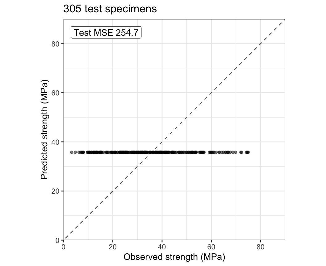
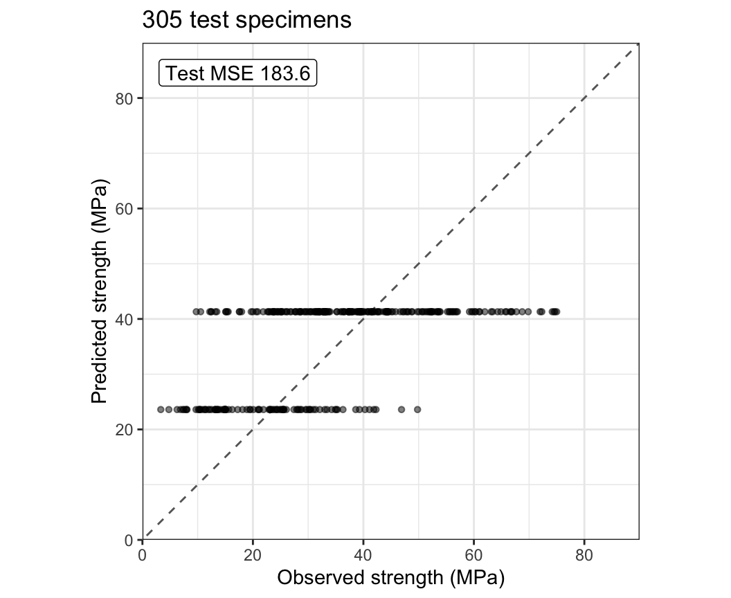
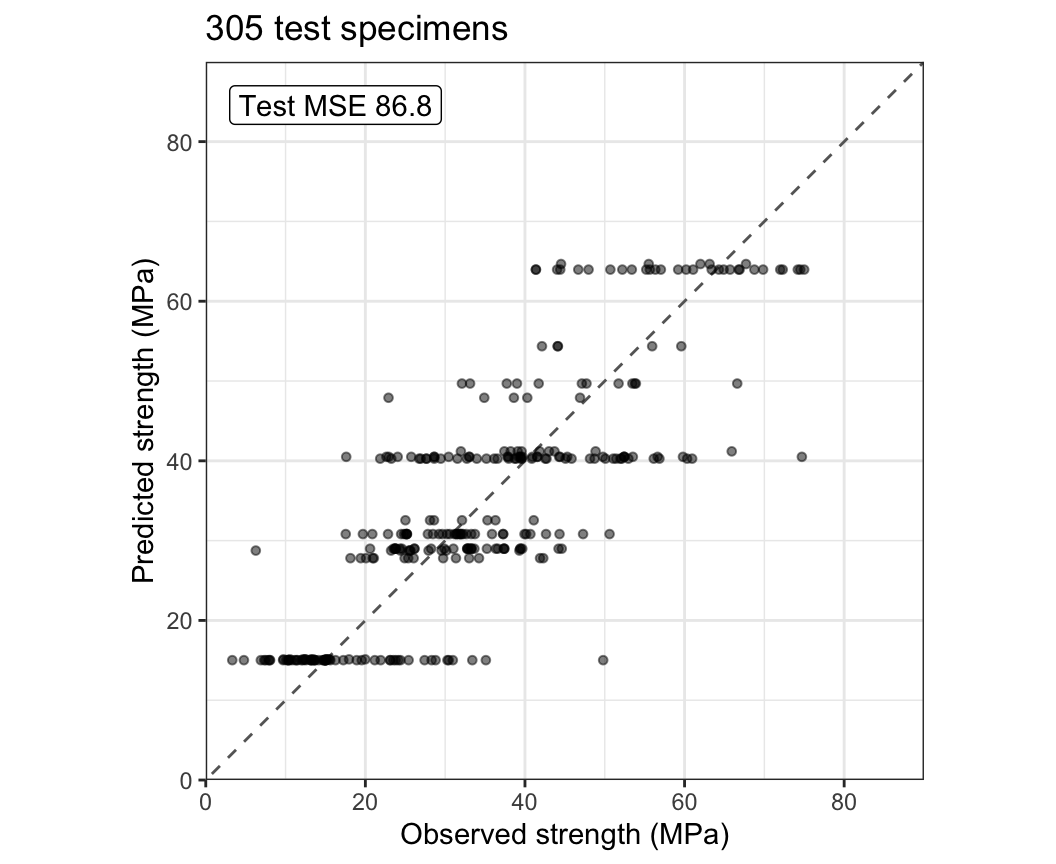
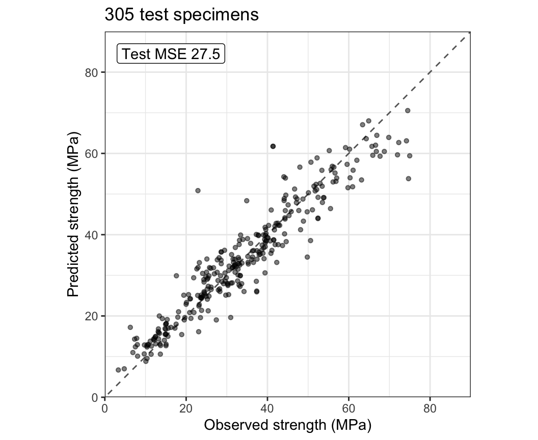
The mean predicts one value for every specimen, the stump 2, and the default tree 15, one per leaf; each horizontal row of points is one leaf or a few leaves with close predictions. Within a leaf the test strengths have a pooled standard deviation of 9.1 MPa, against 15.9 MPa over all the test specimens. The random forest’s predictions follow the dashed line. The test MSEs are 254.7, 183.6, 86.8, and 27.5. The forest here uses \(m = 5\), chosen by its OOB error; bagging (\(m = p\)) has test MSE 26.9. These forests are refit here, so their test MSEs, which depend on random draws, differ from those of the previous lecture by up to 0.8.
A small tree is a poor fit: it predicts a few values, each the mean of many specimens that differ in strength. Bagging and random forests get past this by averaging large trees, each with low bias and high variance. Boosting instead keeps the trees small and adds them up one at a time, each fit to the part of the strength that the trees before it have not yet explained.
29.2 Boosting
- Boosting builds many small trees, one after another.
- Each tree is fit to the residuals of the fit so far, not to the response.
- The prediction is the sum of the trees’ predictions, each multiplied by a small shrinkage, so every tree corrects only part of what is left.
- Each tree learns what the earlier trees missed.
- Three tuning parameters, defined in the Algorithm subsection below, control how the fit builds up: the number of trees \(B\), the shrinkage \(\nu\), and the depth \(\delta\) of each tree.
- Bagging and random forests instead grow their trees independently of one another.
29.2.1 Residuals
Boosting starts from the prediction 0 for every specimen, so its first residuals are the strengths themselves. It fits a small tree to the residuals, adds a shrunken copy of the tree’s predictions to the fit, and recomputes the residuals.
NoteCode
# Explanatory variables of the training and test specimens.
x_train <- select(train, -compressive_strength)
x_test <- select(test, -compressive_strength)

# The loop of the Loop subsection: B trees of depth at most `depth`, each
# grown as far as the depth allows, with shrinkage nu. Returns the trees
# and the training fit after each tree, one column per tree.
depth_control <- function(depth) {
  rpart.control(maxdepth = depth, cp = 0, minsplit = 2, minbucket = 1,
                xval = 0, maxcompete = 0, maxsurrogate = 0)
}
boost_loop <- function(x, y, B, nu, depth) {
  control <- depth_control(depth)
  r <- y
  trees <- vector("list", B)
  train_fit <- matrix(0, nrow(x), B)
  for (b in seq_len(B)) {
    data_b <- mutate(x, r = r)
    trees[[b]] <- rpart(r ~ ., data = data_b, control = control)
    r <- r - nu * predict(trees[[b]], x)
    train_fit[, b] <- y - r
  }
  list(trees = trees, train_fit = train_fit)
}

# The fit of this section and of the Loop subsection: 1,000 trees of
# depth 4 with shrinkage 0.1.
B_loop <- 1000
nu_main <- 0.1
depth_main <- 4
loop_run <- boost_loop(x_train, y_train, B_loop, nu_main, depth_main)

# Residuals of the training specimens after 0, 1, 10, 100, and 1,000
# trees; the tabs name these numbers.
residual_b <- c(0, 1, 10, 100, 1000)
residual_at <- function(b) {
  if (b == 0) {
    return(y_train)
  }
  y_train - loop_run$train_fit[, b]
}

# Ages repeat, so each training specimen's age is jittered once, by up to
# 8% either way, and the jittered age is used in every tab.
age_jit <- train$age * exp(runif(n_train, -0.08, 0.08))

# Age on a log scale: major lines at 1, 2, 5, 10, 20, 50, 100 and 200
# days, no minor lines.
age_axis <- scale_x_log10(breaks = c(1, 2, 5, 10, 20, 50, 100, 200),
                          minor_breaks = NULL,
                          limits = c(0.8, 450),
                          expand = expansion(0))

# Residual: major lines every 20 MPa, minor lines midway.
residual_axis <- scale_y_continuous(breaks = seq(-20, 80, by = 20),
                                    minor_breaks = seq(-10, 90, by = 20),
                                    limits = c(-20, 90),
                                    expand = expansion(0))

# Residuals against age, with the training MSE in a corner.
title_train <- paste(n_train, "training specimens")
residual_plot <- function(b) {
  points <- tibble(age = age_jit, residual = residual_at(b))
  label <- paste("Training MSE", fmt(mean(points$residual^2), 1))
  ggplot(points, aes(x = age, y = residual)) +
    geom_hline(yintercept = 0, color = "grey40") +
    geom_point(alpha = 0.4, size = 1) +
    annotate("label", x = 0.9, y = 87, hjust = 0, vjust = 1,
             label = label) +
    age_axis +
    residual_axis +
    labs(x = "Age (days, log scale)", y = "Residual (MPa)",
         title = title_train)
}
residual_plots <- map(residual_b, residual_plot)
residual_plots <- do.call(patchwork::align_patches, residual_plots)

# Mean fitted value after 10 trees, the largest change one tree makes, and
# the training MSE at the start, after one tree, and after 1,000 trees.
mean_fit_10 <- mean(loop_run$train_fit[, 10])
first_step <- max(abs(loop_run$train_fit[, 1]))
train_mse_0 <- mean(y_train^2)
train_mse_1 <- mean(residual_at(1)^2)
train_mse_1000 <- mean(residual_at(1000)^2)

# A regression tree's predictions for its training data average to the
# mean of its response, so the mean fitted value after b trees is
# 1 - (1 - nu)^b times the mean strength.
level_10 <- 1 - (1 - nu_main)^10
stopifnot(isTRUE(all.equal(mean_fit_10, level_10 * mean(y_train))))

# Correlation of the residuals with log(age), at the start and after 100
# trees.
age_cor <- map_dbl(c(0, 100), \(b) cor(residual_at(b), log(train$age)))
The tabs plot the residuals of the training specimens against age: at the start, the strengths, and then after 1, 10, 100, and 1,000 trees of depth 4 (each leaf reached through at most 4 splits), each tree’s predictions multiplied by the shrinkage \(\nu = 0.1\) before they are added.
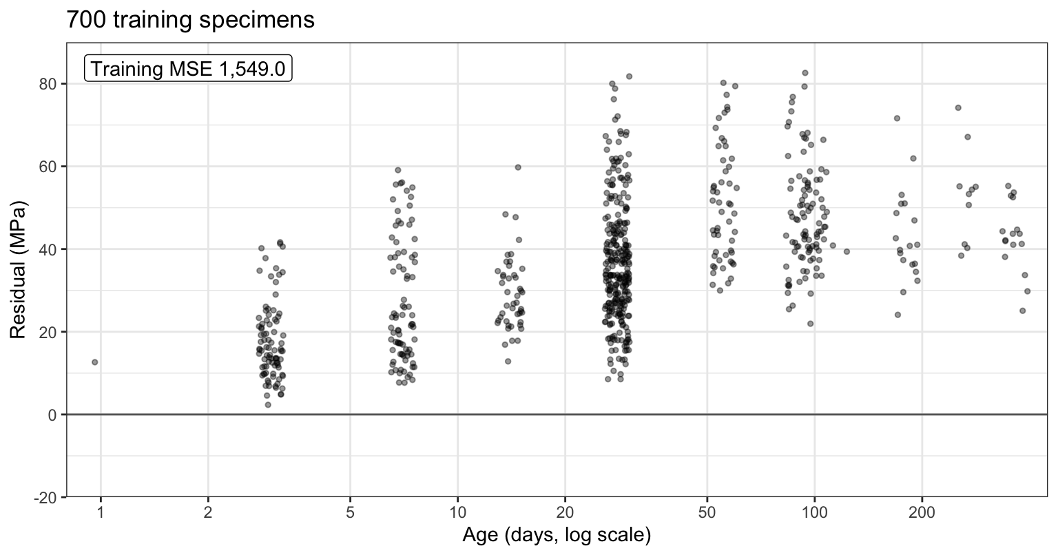
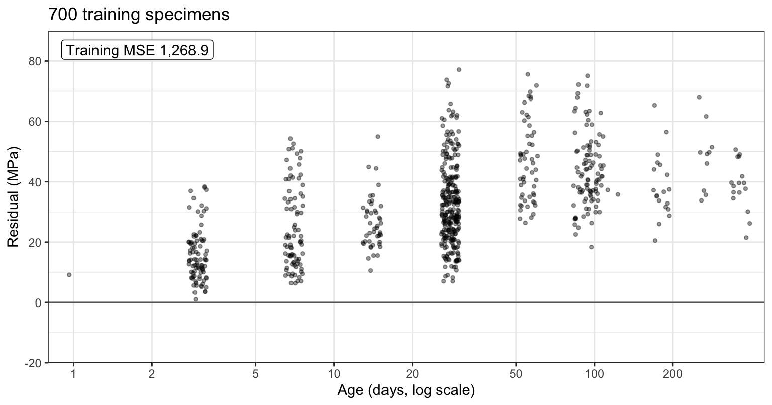
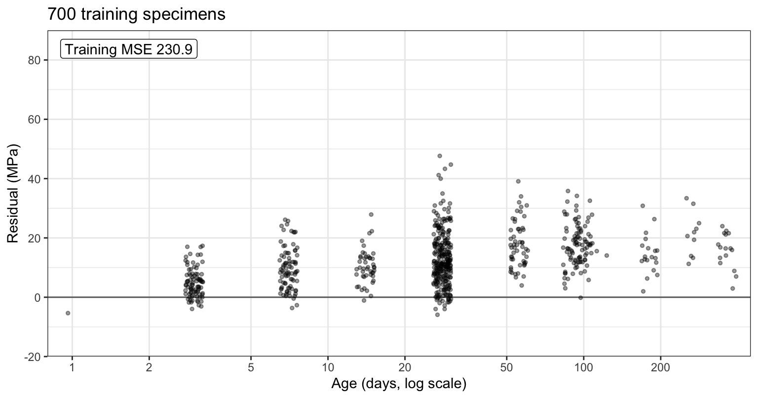
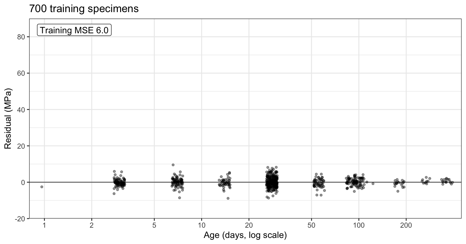
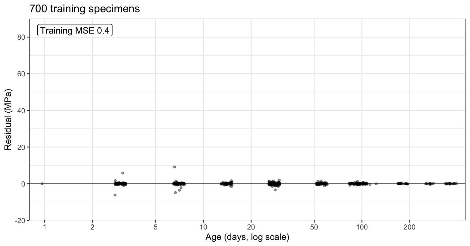
The first tab is the data: strength rises steeply with age over the first month. The fit after one tree is \(\nu = 0.1\) times that tree’s predictions, so no residual moves by more than 7.5 MPa, and the training MSE falls from 1,549.0 to 1,268.9, by 18%. A regression tree’s predictions for its training data average to the mean of the residuals it is fit to, so after \(b\) trees the mean fitted value is \(1 - \left(1 - \nu\right)^b\) times the mean strength. After 10 trees that factor is \(1 - 0.9^{10} = 0.651\): the mean fitted value is 23.3 MPa, against a mean training strength of 35.8, and the first trees mostly raise the overall level from 0. By 100 trees the rise with age is gone from the residuals (their correlation with \(\log(\texttt{age})\) falls from 0.57 to 0.03), and after 1,000 trees the training MSE is 0.42.
29.2.2 Algorithm
Boosting for regression trees, with \(B\) trees of depth \(\delta\) and shrinkage \(\nu\):
- Set \(\hat f_0(x) = 0\) for every \(x\), and \(r_i = y_i\) for every training observation \(i = 1, \ldots, n\).
- For \(b = 1, \ldots, B\):
- fit a tree \(\hat f^b\) of depth \(\delta\) to the training data, with the residuals \(r_1, \ldots, r_n\) as the response;
- add a shrunken copy of it to the fit, \(\hat f_b(x) = \hat f_{b-1}(x) + \nu\,\hat f^b(x)\);
- update the residuals, \(r_i \leftarrow r_i - \nu\,\hat f^b(x_i)\), so that \(r_i = y_i - \hat f_b(x_i)\).
- Predict with the boosted model \[\hat f_B(x) = \sum_{b=1}^B \nu\,\hat f^b(x),\]
where
- \(x_i\) and \(y_i\) are the explanatory variables and the response of training observation \(i\), and \(n\) the number of training observations,
- \(B\) is the number of trees, indexed \(b\), as in the Random Forests lecture,
- \(\hat f^b(x)\) is the prediction at \(x\) of the \(b\)th tree (the superscript names the tree; it has no star, because the tree is not fit to a bootstrap sample),
- \(\hat f_b(x)\) is the boosted model after \(b\) trees, with \(\hat f_0 = 0\),
- \(r_i\) is the current residual of training observation \(i\) (not the lasso residual vector \(r\)),
- \(\nu\), with \(0 < \nu \le 1\), is the shrinkage, or learning rate, which the textbook writes \(\lambda\); in these notes \(\lambda\) is the ridge and lasso tuning parameter, so the shrinkage is \(\nu\), and
- \(\delta\) is the depth of each tree, the largest number of splits on a path from the root to a leaf; \(\delta = 1\) is a stump.
The textbook limits the number of splits, \(d\); in these notes \(d\) is the number of features of the subset selection lectures, and both rpart() and xgboost limit depth, with maxdepth and max_depth. A tree of depth \(\delta\) has at most \(2^\delta\) leaves. The symbol \(\delta\) is unrelated to the discriminant functions \(\delta_k(x)\) of the discriminant analysis lectures and to the interaction estimates \(\delta_j\) of the Flexible Logistic Regression lecture, which always carry a subscript.
The tree at step \(b\) depends on the trees before it through the residuals, so the trees are grown in sequence.
29.2.3 Loop
The chunk writes the algorithm out with rpart(): \(B = 1{,}000\) trees of depth \(\delta = 4\) with shrinkage \(\nu = 0.1\), the fit of the Residuals tabs, on all 8 explanatory variables of the training specimens. The tree settings, small, are set in the callout.
NoteCode
# Trees of depth at most 4, each grown as far as the depth allows.
small <- rpart.control(maxdepth = 4, cp = 0, minsplit = 2, minbucket = 1,
                       xval = 0, maxcompete = 0, maxsurrogate = 0)
# Boosting from scratch: B trees of depth 4, with shrinkage nu.
B <- 1000
nu <- 0.1
# Start from the fit 0, so the residuals are the strengths.
r <- y_train
trees <- vector("list", B)
# Fit a tree to the residuals, then subtract nu times its predictions.
for (b in seq_len(B)) {
data_b <- mutate(x_train, r = r)
trees[[b]] <- rpart(r ~ ., data = data_b, control = small)
r <- r - nu * predict(trees[[b]], x_train)
}cp = 0, minsplit = 2 and minbucket = 1 turn off rpart()‘s other stopping rules, as for the full tree of the Decision Trees lecture, so each tree is grown until its leaves are at depth \(\delta\) or hold specimens that no split separates. xval = 0 skips the cross-validation rpart() would otherwise run, and maxcompete = 0 and maxsurrogate = 0 skip the competing and surrogate splits it would otherwise record, which speeds up the loop without changing any tree. The boosted prediction sums the trees’ predictions and multiplies by \(\nu\):
# Each tree's predictions for the test specimens, one column per tree;
# the boosted prediction is nu times their sum.
tree_pred <- sapply(trees, predict, newdata = test)
boost_pred <- nu * rowSums(tree_pred)
c(train_mse = mean(r^2), test_mse = mean((y_test - boost_pred)^2))
train_mse test_mse
0.4216354 23.6745438
NoteCode
# The loop above is the fit of the Residuals callout.
stopifnot(nu == nu_main,
          B == B_loop,
          small$maxdepth == depth_main,
          isTRUE(all.equal(unname(y_train - r), loop_run$train_fit[, B])))
loop_train <- mean(r^2)
loop_test <- mse(y_test, boost_pred)

# Training specimens in the leaves of the first tree of the loop.
first_leaf_n <- with(trees[[1]]$frame, n[var == "<leaf>"])
first_leaf_min <- min(first_leaf_n)
first_leaf_max <- max(first_leaf_n)
The leaves of the first tree hold 6 to 161 training specimens. With \(B = 1{,}000\) trees the training MSE is 0.42 and the test MSE 23.7, against 86.8 for the default tree and 27.5 for the random forest.
29.3 xgboost
29.3.1 Fitting
NoteCode
# xgboost's defaults, read from the settings of a one-tree fit with no
# tuning parameters set.
default_fit <- xgb.train(xgb.params(nthread = 1),
                         xgb.DMatrix(x_train, label = y_train, nthread = 1),
                         nrounds = 1)
default_config <- xgb.config(default_fit)$learner
tree_param <- default_config$gradient_booster$tree_train_param
xgb_default <- map(tree_param[c("eta", "max_depth", "lambda", "max_bin",
                                "min_child_weight", "gamma")],
                   \(value) signif(as.numeric(value), 3))

# The start, base_score, is the mean training strength (stored in single
# precision), and the default split search is the histogram method.
base_score <- default_config$learner_model_param$base_score
base_score <- as.numeric(gsub("[][]", "", base_score))
default_updater <- default_config$gradient_booster$updater$name
stopifnot(abs(base_score - mean(y_train)) < 1e-4,
          default_updater == "grow_quantile_histmaker",
          xgb_default$min_child_weight == 1,
          xgb_default$gamma == 0)
The xgboost package fits boosted trees in compiled code. Its arguments name this lecture’s tuning parameters differently:
learning_rate(or its aliaseta) is the shrinkage \(\nu\), by default 0.3;max_depthis the depth \(\delta\), by default 6;nroundsis the number of trees \(B\), one per round, with no default.
xgb.DMatrix() stores the explanatory variables with the response, xgb.params() collects the tuning parameters, and xgb.train() fits the model, with the squared-error loss by default for a numeric response. nthread = 1 runs it on one processor thread. The chunk fits the loop’s \(\nu\), \(\delta\) and \(B\).
# The training and test data in xgboost's format.
x_test <- select(test, -compressive_strength)
d_train <- xgb.DMatrix(x_train, label = y_train, nthread = 1)
d_test <- xgb.DMatrix(x_test, label = y_test, nthread = 1)

# B = 1,000 trees of depth 4 with shrinkage 0.1, and the test MSE.
params <- xgb.params(learning_rate = 0.1, max_depth = 4, nthread = 1)
fit <- xgb.train(params, d_train, nrounds = 1000)
mean((y_test - predict(fit, d_test))^2)
[1] 24.0684
NoteCode
# The fit's training and test MSE, and its tuning parameters, which are
# those of the loop.
xgb_train <- mse(y_train, predict(fit, d_train))
xgb_test <- mse(y_test, predict(fit, d_test))
stopifnot(params$learning_rate == nu_main,
          params$max_depth == depth_main,
          xgb.get.num.boosted.rounds(fit) == B_loop)
The test MSE is 24.1, against 23.7 for the loop: the two fits use the same \(\nu\), \(\delta\) and \(B\), but are not the same model.
29.3.2 Loop reproduction
xgboost differs from the loop in three ways, each a default:
- Start. It starts from the mean training strength (its
base_score), not from 0. - Leaf predictions. It grows each tree from the first and second derivatives of the loss at the current fit. For the squared-error loss \(\tfrac{1}{2}\left[y_i - \hat f_{b-1}(x_i)\right]^2\) these are \(-r_i\) and \(1\), so the tree is fit to the residuals, as in the loop, but a leaf predicts, before the shrinkage \(\nu\), \[\frac{\sum_{i \in \text{leaf}} r_i}{n_{\text{leaf}} + \texttt{lambda}},\] where
- the sum runs over the training specimens in the leaf,
- \(n_{\text{leaf}}\) is their number, and
lambda, by default 1, is a penalty that shrinks the leaf’s prediction toward 0, as ridge regression shrinks its estimates (lambdaisxgboost’s name; it is not the ridge \(\lambda\) of these notes).
lambda = 0the leaf predicts the mean of its residuals, as anrpart()leaf does. - Split search. By default (
tree_method = "hist") it groups each explanatory variable’s values into at most 256 bins and tries cut points only between bins, not between every pair of adjacent values.
Setting lambda = 0, base_score = 0 and tree_method = "exact" removes all three. The other defaults already match the loop: every leaf holds at least one specimen (min_child_weight = 1, minbucket = 1), and any decrease in RSS justifies a split (gamma = 0, cp = 0).
# xgboost with the loop's start, leaf predictions, and split search.
loop_params <- xgb.params(learning_rate = 0.1, max_depth = 4, nthread = 1,
                          lambda = 0, base_score = 0, tree_method = "exact")
loop_fit <- xgb.train(loop_params, d_train, nrounds = 1000)

# The training fits of the loop and of xgboost after 200 trees.
loop_200 <- nu * rowSums(sapply(trees[1:200], predict, newdata = x_train))
xgb_200 <- predict(loop_fit, d_train, iterationrange = c(1, 200))
max(abs(loop_200 - xgb_200))
[1] 6.576375e-05
NoteCode
# Each tree of the loop-settings fit against the same tree of the loop:
# the largest gap between nu times their predictions, for the training
# and the test specimens.
tree_gap <- function(b, d, x) {
  xgb_tree <- predict(loop_fit, d, iterationrange = c(b, b))
  max(abs(xgb_tree - nu * predict(trees[[b]], x)))
}
train_tree_gaps <- map_dbl(seq_len(B), \(b) tree_gap(b, d_train, x_train))
test_tree_gaps <- map_dbl(seq_len(B), \(b) tree_gap(b, d_test, x_test))

# The first tree that differs on the training specimens, the first that
# differs on the test specimens only, and the number of trees before the
# first that differ on the test specimens only.
gap_tol <- 1e-3
first_train_differ <- which(train_tree_gaps > gap_tol)[1]
first_test_differ <- which(test_tree_gaps > gap_tol)[1]
before_split <- seq(first_test_differ, first_train_differ - 1)
n_test_only <- sum(test_tree_gaps[before_split] > gap_tol)
gap_200 <- max(abs(loop_200 - xgb_200))
stopifnot(first_train_differ > 200,
          first_test_differ < first_train_differ,
          gap_200 < gap_tol)

# The splits of a tree of each program: variable, number of training
# specimens in the node, and cut point (rounded, since xgboost stores it in
# single precision).
rpart_splits <- function(tree) {
  tibble(var = rownames(tree$splits),
         n = tree$splits[, "count"],
         cut = round(tree$splits[, "index"], 2))
}
xgb_splits <- function(b) {
  xgb.model.dt.tree(loop_fit, trees = b) |>
    as_tibble() |>
    filter(Feature != "Leaf") |>
    transmute(var = Feature, n = Cover, cut = round(Split, 2))
}

# In the first tree that differs on the test specimens, the splits found
# in one program only, largest node first: here a pair at the root, on the
# same variable with different cut points, and a pair in a node of a few
# specimens, on different variables.
b_test <- first_test_differ
rpart_only <- anti_join(rpart_splits(trees[[b_test]]), xgb_splits(b_test),
                        by = c("var", "n", "cut")) |>
  arrange(desc(n))
xgb_only <- anti_join(xgb_splits(b_test), rpart_splits(trees[[b_test]]),
                      by = c("var", "n", "cut")) |>
  arrange(desc(n))
stopifnot(nrow(rpart_only) == 2, nrow(xgb_only) == 2,
          all(rpart_only$n == xgb_only$n),
          rpart_only$n[1] == n_train,
          rpart_only$var[1] == xgb_only$var[1],
          rpart_only$var[2] != xgb_only$var[2])

# The two root cut points make the same partition of the training
# specimens, and no test specimen lies between them.
root_var <- rpart_only$var[1]
root_cuts <- c(rpart_only$cut[1], xgb_only$cut[1])
between <- function(x) {
  x >= min(root_cuts) & x < max(root_cuts)
}
stopifnot(!any(between(train[[root_var]])),
          !any(between(test[[root_var]])))

# Test specimens whose prediction from that tree differs.
n_test_moved <- sum(abs(predict(loop_fit, d_test,
                                iterationrange = c(b_test, b_test)) -
                          nu * tree_pred[, b_test]) > gap_tol)

# The first tree that differs on the training specimens: both split the
# root the same way; in the larger child, the gains (decreases in RSS) of
# the loop's split and of xgboost's split, computed with the loop's
# residuals and with xgboost's (single-precision) residuals before it.
b_train <- first_train_differ
rpart_b <- rpart_splits(trees[[b_train]])
xgb_b <- xgb_splits(b_train)
stopifnot(rpart_b$var[1] == xgb_b$var[1],
          rpart_b$cut[1] == xgb_b$cut[1])
node <- x_train[[rpart_b$var[1]]] >= rpart_b$cut[1]
node_n <- sum(node)
candidates <- bind_rows(filter(rpart_b, n == node_n)[1, ],
                        filter(xgb_b, n == node_n)[1, ])
node_gain <- function(residual, var, cut) {
  left <- x_train[[var]][node] < cut
  res <- residual[node]
  sum(res[left])^2 / sum(left) + sum(res[!left])^2 / sum(!left) -
    sum(res)^2 / length(res)
}
residual_loop <- y_train - loop_run$train_fit[, b_train - 1]
residual_xgb <- y_train -
  predict(loop_fit, d_train, iterationrange = c(1, b_train - 1))
gain_loop <- map2_dbl(candidates$var, candidates$cut,
                      \(v, cut) node_gain(residual_loop, v, cut))
gain_xgb <- map2_dbl(candidates$var, candidates$cut,
                     \(v, cut) node_gain(residual_xgb, v, cut))

# The prose says the loop's residuals favor the loop's split and xgboost's
# favor xgboost's.
stopifnot(candidates$var[1] != candidates$var[2],
          gain_loop[1] > gain_loop[2],
          gain_xgb[2] > gain_xgb[1])
gain_fmt <- function(x) {
  formatC(x, format = "f", digits = 6)
}

# The three fits, each with 1,000 trees of depth 4 and shrinkage 0.1.
loop_fit_train <- predict(loop_fit, d_train)
loop_fit_test <- predict(loop_fit, d_test)
reproduction <- tribble(
  ~Fit, ~Settings, ~train, ~test,
  "Loop of rpart() fits", "start at 0", loop_train, loop_test,
  "xgboost, loop settings",
  "`lambda = 0`, `base_score = 0`, `tree_method = \"exact\"`",
  mse(y_train, loop_fit_train), mse(y_test, loop_fit_test),
  "xgboost, defaults",
  paste0("`lambda = ", xgb_default$lambda,
         "`, start at the mean, `tree_method = \"hist\"`"),
  xgb_train, xgb_test
) |>
  mutate(train = fmt(train, 2), test = fmt(test, 1))
reproduction_table <- knitr::kable(reproduction,
                                   col.names = c("Fit", "Settings",
                                                 "Training MSE",
                                                 "Test MSE"),
                                   align = "llrr")
iterationrange = c(1, 200) predicts with trees 1 to 200 (counted from 1, both ends included). With the loop’s settings, xgboost reproduces the loop to rounding through tree 232, and not after:
- Training fits. After 200 trees the two training fits differ by at most 0.00007 MPa, a rounding difference, since
xgboostcomputes in single precision. - Test predictions. Of trees 20 to 232, 32 predict differently, by more than 0.001 MPa, for some test specimen while agreeing on every training specimen: in a node, both programs make the same partition of the training specimens with a different split. In tree 20, both split the root at the same place in
age,rpart()cutting at 10.5 andxgboostat 11, with no specimen in between; deeper, both separate the same 2 training specimens from the rest of a node,rpart()withwaterat 201.75 andxgboostwithcementat 275.4, which sends 1 test specimen to a different leaf. - Tree 233. Both split the root on
ageat 2. In the node of the other 699 training specimens two splits nearly tie. With the loop’s residuals,ageat 42 decreases the RSS by 0.624287 andfine_aggregateat 884.65 by 0.624186, sorpart()takes the first; withxgboost’s residuals, which differ from the loop’s by rounding, the decreases are 0.624227 and 0.624234, soxgboosttakes the second. From there the trees differ.
The table compares the three fits after 1,000 trees.
| Fit | Settings | Training MSE | Test MSE |
|---|---|---|---|
| Loop of rpart() fits | start at 0 | 0.42 | 23.7 |
| xgboost, loop settings | lambda = 0, base_score = 0, tree_method = "exact" |
0.41 | 25.0 |
| xgboost, defaults | lambda = 1, start at the mean, tree_method = "hist" |
0.58 | 24.1 |
The rest of this lecture uses xgboost with its defaults, apart from \(\nu\), \(\delta\) and \(B\).
29.4 Tuning parameters
Boosting has three tuning parameters:
- the number of trees \(B\) (
nrounds), how many trees are added; - the shrinkage \(\nu\) (
learning_rate), the multiplier of each tree’s predictions before they are added, which sets how fast the model learns; - the depth \(\delta\) (
max_depth), the largest number of splits on a path from the root to a leaf, which sets how complex each tree is.
xgboost has further settings, among them lambda, min_child_weight and gamma of the Loop reproduction subsection and subsample, the share of the training specimens each tree is fit to; this lecture leaves them at their defaults.
The Shrinkage, Tree depth and Overfitting figures plot the test MSE against the number of trees to show what each tuning parameter does. They use the test specimens for teaching only and choose nothing: \(\nu = 0.1\) and \(\delta = 4\) were fixed in advance, and the model fit for the rest of the lecture uses them. In practice every tuning parameter is chosen without the test data, by cross-validation (or, for a forest, by out-of-bag error), as \(B\) is in the Cross-validation estimate subsection.
29.4.1 Shrinkage
NoteCode
# Training and test MSE after each number of trees, from xgboost's
# evaluation log, for shrinkage nu and depth `depth`, with the fit.
B_max <- 5000
curve_run <- function(nu, depth) {
  run_params <- xgb.params(learning_rate = nu, max_depth = depth,
                           nthread = 1)
  run_fit <- xgb.train(run_params, d_train, nrounds = B_max,
                       evals = list(train = d_train, test = d_test),
                       verbose = 0)
  log <- attributes(run_fit)$evaluation_log
  curve <- tibble(nu = nu, depth = depth, trees = log$iter,
                  train = log$train_rmse^2, test = log$test_rmse^2)
  list(fit = run_fit, curve = curve)
}

# Three shrinkages at depth 4.
nu_values <- c(0.5, 0.1, 0.01)
shrink_runs <- map(nu_values, \(v) curve_run(v, depth_main))
shrink_curves <- list_rbind(map(shrink_runs, "curve"))

# The curve for nu = 0.1 extends the fit of the Fitting subsection.
main_index <- which(nu_values == nu_main)
main_test <- filter(shrink_curves, nu == nu_main)$test
stopifnot(abs(main_test[B_loop] - xgb_test) < 1e-3)

# The smallest test MSE of each curve, where it is, and the test MSE at
# B_max trees.
shrink_min <- shrink_curves |>
  slice_min(test, n = 1, with_ties = FALSE, by = nu) |>
  select(nu, trees, test)
shrink_at <- function(v, column = "test", b = B_max) {
  filter(shrink_curves, nu == v, trees == b)[[column]]
}
min_of <- function(v, column = "test") {
  filter(shrink_min, nu == v)[[column]]
}

# A curve is still falling at B_max when its smallest value is in the last
# 10% of the trees; its smallest value is then not a minimum.
falling_after <- function(min_trees) {
  min_trees > 0.9 * B_max
}
small_nu <- min(nu_values)
still_falling <- falling_after(min_of(small_nu, "trees"))
small_nu_text <- if (still_falling) {
  "and still falling"
} else {
  paste("its smallest value", fmt(min_of(small_nu), 1), "after",
        big(min_of(small_nu, "trees")))
}

# Number of trees on a log scale: the 1-2-5 pattern from 1 to 5,000, no
# minor lines.
trees_axis <- scale_x_log10(breaks = c(1, 2, 5, 10, 20, 50, 100, 200, 500,
                                       1000, 2000, 5000),
                            minor_breaks = NULL,
                            labels = scales::label_comma())

# Test MSE: major lines every 10, minor lines midway; the first trees,
# far above, are clipped.
curve_axis <- scale_y_continuous(breaks = seq(20, 50, by = 10),
                                 minor_breaks = seq(15, 55, by = 10))
curve_ylim <- c(15, 55)
curve_caption <- paste("Dashed line: the random forest.",
                       "Circles: the smallest test MSE of each curve.",
                       "Values above", curve_ylim[2], "are clipped.")

# Test MSE curves by a tuning parameter, with the forest's test MSE and the
# smallest value of each curve circled. The curves are drawn and labeled in
# the order of `levels`; `labels` (plotmath expressions or text) go with
# `levels` in that order.
curve_plot <- function(curves, minima, group, levels, labels, colors) {
  curves <- mutate(curves, group = factor(.data[[group]], levels = levels))
  linetypes <- c("solid", "longdash", "dotted", "dotdash")
  ggplot(curves, aes(x = trees, y = test, color = group,
                     linetype = group)) +
    geom_hline(yintercept = forest_mse[["forest"]], linetype = "dashed",
               color = "grey40") +
    geom_line() +
    geom_point(data = minima, aes(x = trees, y = test),
               inherit.aes = FALSE, size = 4, shape = 1) +
    scale_color_manual(values = colors[seq_along(levels)],
                       breaks = as.character(levels), labels = labels) +
    scale_linetype_manual(values = linetypes[seq_along(levels)],
                          breaks = as.character(levels), labels = labels) +
    trees_axis +
    curve_axis +
    coord_cartesian(ylim = curve_ylim) +
    labs(x = "Number of trees b (log scale)", y = "Test MSE (MPa squared)",
         color = NULL, linetype = NULL, title = title_train,
         caption = curve_caption) +
    theme(legend.position = "inside",
          legend.position.inside = c(0.99, 0.97),
          legend.justification = c(1, 1),
          legend.background = element_rect(color = "grey50"))
}
nu_labels <- parse(text = paste("nu ==", nu_values))
shrink_plot <- curve_plot(shrink_curves, shrink_min, "nu", nu_values,
                          nu_labels, okabe_ito[c(4, 5, 3)])

# Test MSE after 100 trees, by shrinkage, and of the mean training
# strength, xgboost's start.
mse_100 <- map_dbl(nu_values, \(v) shrink_at(v, "test", 100)) |>
  set_names(nu_values)
mse_start <- earlier_test[["Mean"]]

# The prose says a smaller nu reaches its smallest test MSE after more
# trees, and that after 100 trees nu = 0.01 is closer to the start than
# nu = 0.1.
stopifnot(!is.unsorted(map_dbl(nu_values, \(v) min_of(v, "trees"))),
          mse_100[["0.01"]] > mse_100[["0.1"]],
          mse_100[["0.01"]] < mse_start,
          small_nu == 0.01, nu_values[2] == nu_main)
The figure plots the test MSE of the boosted model after \(b\) trees against \(b\), for \(\nu = 0.5\), \(\nu = 0.1\), and \(\nu = 0.01\), each with trees of depth \(\delta = 4\), with the random forest’s test MSE as a dashed line. xgb.train() records these with evals = list(train = d_train, test = d_test): the MSE of each data set after every round, kept as the RMSE in the fit’s evaluation_log.
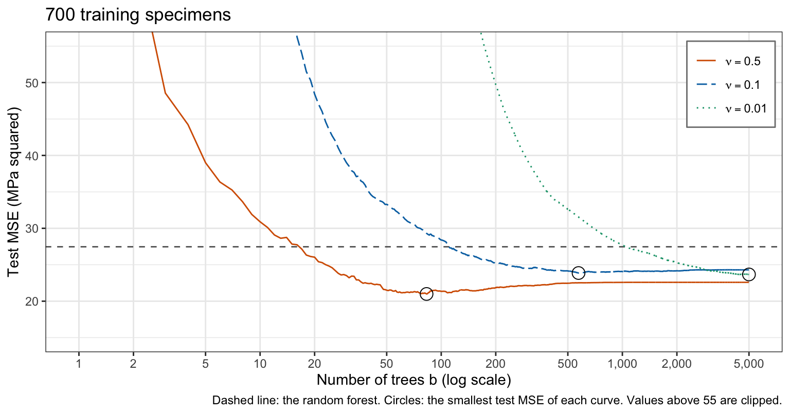
The smaller the shrinkage, the more trees the model needs. With \(\nu = 0.5\) the test MSE is smallest, 21.0, after 83 trees; with \(\nu = 0.1\) it is smallest, 23.9, after 573; with \(\nu = 0.01\) it is 23.7 after 5,000 trees, and still falling. After 100 trees the test MSE is 85.9 with \(\nu = 0.01\) and 28.4 with \(\nu = 0.1\), against 254.7 for the mean training strength, xgboost’s starting point. As a large \(\lambda\) does in ridge regression and the lasso, a small \(\nu\) holds the fit near its starting point, and more trees let it move further from it.
29.4.2 Tree depth
NoteCode
# Test MSE after each number of trees, for four depths at nu = 0.1; the
# Shrinkage fits supply depth 4.
depth_values <- c(1, 2, 4, 8)
depth_runs <- map(depth_values, \(d) {
  if (d == depth_main) {
    shrink_runs[[main_index]]
  } else {
    curve_run(nu_main, d)
  }
})
depth_curves <- list_rbind(map(depth_runs, "curve"))
depth_min <- depth_curves |>
  slice_min(test, n = 1, with_ties = FALSE, by = depth) |>
  select(depth, trees, test)
depth_at <- function(d, column = "test") {
  filter(depth_min, depth == d)[[column]]
}

# The depth with the smallest test MSE over all numbers of trees.
best_depth <- depth_min$depth[which.min(depth_min$test)]
depth_labels <- parse(text = paste("delta ==", depth_values))

# Test MSE at B_max trees and 1,000 trees earlier, by depth, and which
# curves are still falling at B_max.
depth_end <- function(d, b = B_max) {
  filter(depth_curves, depth == d, trees == b)$test
}
depth_min_trees <- map_dbl(depth_values, \(d) depth_at(d, "trees"))
depth_falling <- set_names(falling_after(depth_min_trees), depth_values)
falling_depths <- depth_values[depth_falling]
last_drop <- map_dbl(falling_depths, \(d) {
  depth_end(d, B_max - 1000) - depth_end(d)
})
falling_text <- if (length(falling_depths) == 0) {
  "Every curve reaches its smallest value before the last trees."
} else {
  paste0("The ",
         if (length(falling_depths) == 1) "curve" else "curves",
         if (length(falling_depths) == 1) " for depth " else " for depths ",
         and_list(falling_depths),
         if (length(falling_depths) == 1) " is" else " are",
         " still falling at ", big(B_max), " trees, but slowly: the last ",
         "1,000 trees lowered ",
         if (length(falling_depths) == 1) "it" else "them",
         " by ", and_list(fmt(last_drop, 1)), ".")
}

# How far the deepest trees' curve rises from its smallest value, and how
# the prose describes it.
deep <- max(depth_values)
deep_rise <- depth_end(deep) / depth_at(deep) - 1
deep_text <- if (deep_rise < 0.01) {
  paste0("then stays within 1% of it up to ", big(B_max), " trees")
} else {
  paste0("then rises ", pct(deep_rise, 0), " by ", big(B_max), " trees")
}

# The prose says stumps are still falling at B_max; that deeper trees
# reach their smallest test MSE after fewer trees; that the deepest
# trees reach theirs first; and that the stumps at B_max do worse than the
# smallest value of every larger depth.
stopifnot(depth_falling[["1"]],
          !is.unsorted(rev(depth_min_trees)),
          deep_rise >= 0,
          depth_end(1) > max(map_dbl(depth_values[-1], depth_at)))
depth_plot <- curve_plot(depth_curves, depth_min, "depth", depth_values,
                         depth_labels, okabe_ito[c(1, 4, 5, 3)])
The figure plots the test MSE against the number of trees for depths \(\delta = 1\), \(\delta = 2\), \(\delta = 4\), and \(\delta = 8\), each with \(\nu = 0.1\).
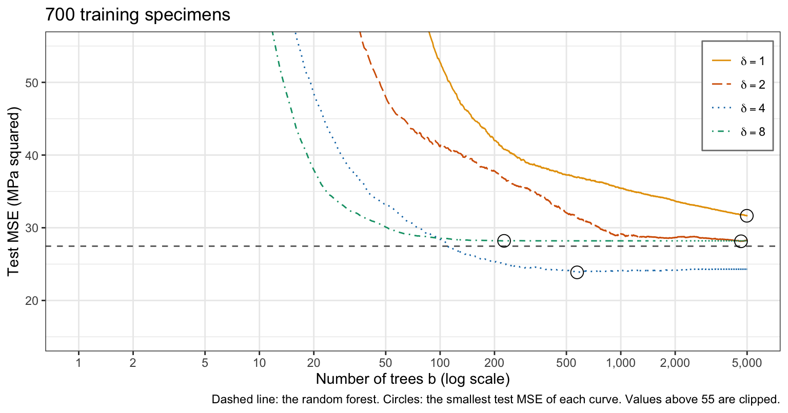
Deeper trees learn faster. The test MSE is smallest after 226 trees of depth 8 (28.2), 573 of depth 4 (23.9), and 4,626 of depth 2 (28.1). The curves for depths 1 and 2 are still falling at 5,000 trees, but slowly: the last 1,000 trees lowered them by 0.4 and 0.1. Depth 4 has the smallest test MSE, and depth 8 reaches its smallest value first and then stays within 1% of it up to 5,000 trees. The Additive structure section shows what the depth changes in the fitted model: the interactions it can represent.
29.4.3 Overfitting
NoteCode
# The test MSE curves for nu = 0.5 and 0.1 at depth 4, on a linear axis.
over_nu <- c(0.5, 0.1)
over_curves <- filter(shrink_curves, nu %in% over_nu) |>
  mutate(nu = factor(nu, levels = over_nu))
over_min <- filter(shrink_min, nu %in% over_nu)

# How far each curve rises from its smallest value to B_max trees.
rise <- map_dbl(over_nu, \(v) shrink_at(v) / min_of(v) - 1) |>
  set_names(over_nu)

# Training and test MSE after B_max trees with nu = 0.5.
train_end <- shrink_at(0.5, "train")
test_end <- shrink_at(0.5)

# Training specimens that share all eight explanatory variables with
# another training specimen. No tree separates them, so the training MSE
# cannot fall below the spread of their strengths about their group
# means.
same_x <- train |>
  mutate(group = cur_group_id(), .by = all_of(explanatory)) |>
  filter(n() > 1, .by = group)
floor_mse <- same_x |>
  mutate(deviation = compressive_strength - mean(compressive_strength),
         .by = group) |>
  summarise(floor = sum(deviation^2) / n_train) |>
  pull(floor)
stopifnot(train_end >= floor_mse,
          train_end / floor_mse - 1 < 0.01)

# The number of trees after which the training MSE with nu = 0.5 stays
# within 1% of its value at B_max.
flat_from <- shrink_curves |>
  filter(nu == 0.5) |>
  mutate(off = abs(train / train_end - 1) > 0.01) |>
  summarise(trees = max(trees[off]) + 1) |>
  pull(trees)

# For comparison, the test MSE of the bagging forest of the Earlier fits
# after 50 to all of its trees: the average of its first b trees.
bag_individual <- predict(bag_rf, test, predict.all = TRUE)$individual
bag_running <- t(apply(bag_individual, 1, cumsum)) /
  matrix(seq_len(bag_rf$ntree), nrow(test), bag_rf$ntree, byrow = TRUE)
bag_curve <- colMeans((y_test - bag_running)^2)
bag_late <- range(bag_curve[50:bag_rf$ntree])

# The prose says both curves rise after their smallest value, the curve for
# the smaller nu less.
stopifnot(all(rise > 0), rise[["0.1"]] < rise[["0.5"]])

# Number of trees: major lines every 1,000, minor lines midway. Test MSE:
# major lines every 2, minor lines midway; the first trees are clipped.
over_ylim <- c(20, 30)
over_plot <- ggplot(over_curves,
                    aes(x = trees, y = test, color = nu, linetype = nu)) +
  geom_line() +
  geom_point(data = over_min, aes(x = trees, y = test),
             inherit.aes = FALSE, size = 4, shape = 1) +
  scale_color_manual(values = okabe_ito[c(4, 5)],
                     breaks = as.character(over_nu),
                     labels = nu_labels[1:2]) +
  scale_linetype_manual(values = c("solid", "longdash"),
                        breaks = as.character(over_nu),
                        labels = nu_labels[1:2]) +
  scale_x_continuous(breaks = seq(0, 5000, by = 1000),
                     minor_breaks = seq(500, 4500, by = 1000),
                     labels = scales::label_comma()) +
  scale_y_continuous(breaks = seq(20, 30, by = 2),
                     minor_breaks = seq(21, 29, by = 2)) +
  coord_cartesian(ylim = over_ylim) +
  labs(x = "Number of trees b", y = "Test MSE (MPa squared)",
       color = NULL, linetype = NULL, title = title_train,
       caption = paste("Circles: the smallest test MSE of each curve.",
                       "Values above", over_ylim[2], "are clipped.")) +
  theme(legend.position = "inside",
        legend.position.inside = c(0.99, 0.97),
        legend.justification = c(1, 1),
        legend.background = element_rect(color = "grey50"))
The figure plots the test MSE for \(\nu = 0.5\) and \(\nu = 0.1\), at depth 4, against the number of trees on a linear axis, from the same fits as the Shrinkage figure.
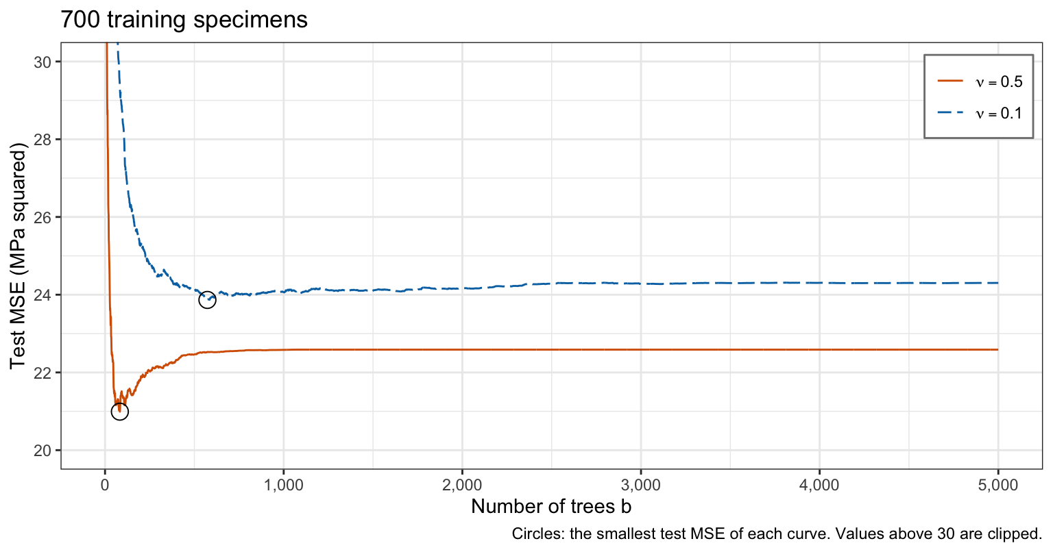
Both curves reach a smallest value and then rise. With \(\nu = 0.5\), the test MSE rises 8% from its smallest value, after 83 trees, to 5,000 trees; with \(\nu = 0.1\) it rises 2% from its smallest value, after 573 trees. The training MSE with \(\nu = 0.5\) falls to 0.28 and stays there from about 583 trees on, while its test MSE is 22.6: the late trees fit what is left of the training residuals, which does not carry over to the test specimens. That training MSE is within 1% of the smallest any model of these explanatory variables can reach, 0.28: 11 training specimens share all 8 explanatory variables with another training specimen of a different strength, and no split separates them. Bagging’s test error levels off instead: the bagging forest of the Earlier fits has test MSE between 26.5 and 27.8 from 50 to its 500 trees. Boosting overfits when \(B\) is too large; a smaller \(\nu\) makes the rise slower.
29.4.4 Cross-validation estimate
\(B\) is chosen like any tuning parameter, by cross-validation, without the test data, here 10-fold, with \(\nu = 0.1\) and \(\delta = 4\) fixed. Split the training observations at random into 10 folds of equal size; for each fold \(\ell\), run boosting on the other nine folds and record the error on fold \(\ell\) after every number of trees. The estimate for \(B\) trees is
\[\text{CV}_{(10)}(B) = \frac{1}{10}\sum_{\ell=1}^{10}\text{MSE}_\ell(B), \qquad \text{MSE}_\ell(B) = \frac{1}{n_\ell}\sum_{i \in \mathcal{F}_\ell}\left[y_i - \hat f_B^{(-\ell)}(x_i)\right]^2,\]
where
- \(\mathcal{F}_\ell\) is the set of training observations in fold \(\ell\), and \(n_\ell\) their number, here \(n/10\),
- \(\hat f_B^{(-\ell)}\) is the boosted model of \(B\) trees fit to the observations outside fold \(\ell\), and
- \(\text{MSE}_\ell(B)\) is its MSE on fold \(\ell\).
One run of \(B_{\max}\) trees per fold gives the estimate for every \(B \le B_{\max}\), because the model of \(B\) trees is the first \(B\) trees of the longer run. xgb.cv() does this: it grows the models of the 10 folds side by side and records, after every round, the mean and the standard deviation over the folds of the RMSE, the root of the fold’s MSE, as test_rmse_mean and test_rmse_std (xgboost’s word test there names the held-out fold, not the test specimens). The mean of the squares is the square of the mean plus the variance with divisor 10, so
\[\text{CV}_{(10)}(B) = \frac{1}{10}\sum_{\ell=1}^{10}\text{RMSE}_\ell(B)^2 = \overline{\text{RMSE}}(B)^2 + \frac{9}{10}\,s_{\text{RMSE}}(B)^2,\]
where
- \(\text{RMSE}_\ell(B)\) is the root mean squared error on fold \(\ell\),
- \(\overline{\text{RMSE}}(B)\) is
test_rmse_mean, the mean over the folds of \(\text{RMSE}_\ell(B)\), and - \(s_{\text{RMSE}}(B)\) is
test_rmse_std, their standard deviation with divisor \(10 - 1 = 9\).
Two notes on this second form:
- It holds only when the folds have equal size, here 70 training specimens each. With unequal folds the estimate is the weighted average of the fold MSEs, \(\sum_{\ell} (n_\ell / n)\,\text{MSE}_\ell(B)\), the first display with weights \(n_\ell / n\) in place of \(1/10\), and the second form does not hold.
- It is used here because
xgb.cv()records only the mean and the standard deviation of the fold RMSEs.
Here \(B_{\max} = 5{,}000\), and the run uses the params of the Fitting subsection. The folds are drawn with R’s random numbers, so the seed set at the start of the lecture fixes them.
# 10-fold cross-validation for every number of trees up to 5,000.
cv_fit <- xgb.cv(params, d_train, nrounds = 5000, nfold = 10, verbose = 0)
cv_log <- cv_fit$evaluation_log

# The CV estimate of the test MSE after each number of trees; the best B.
cv_mse <- cv_log$test_rmse_mean^2 + 0.9 * cv_log$test_rmse_std^2
B_cv <- which.min(cv_mse)
c(B = B_cv, cv = cv_mse[B_cv])
B cv
1194.00000 20.03447
NoteCode
# The run is B_max trees long, with 10 folds of 70 training specimens.
fold_sizes <- lengths(cv_fit$folds)
stopifnot(nrow(cv_log) == B_max,
          all(fold_sizes == n_train / 10))

# The second display, checked once on these equal folds: pooling the
# out-of-fold predictions of a short run on the same folds gives the same
# estimate.
check_rounds <- 20
check_fit <- xgb.cv(params, d_train, nrounds = check_rounds,
                    folds = cv_fit$folds, prediction = TRUE, verbose = 0)
pooled_mse <- mse(y_train, check_fit$cv_predict$pred)
stopifnot(abs(pooled_mse - cv_mse[check_rounds]) < 1e-3)

# The chosen B's cross-validation estimate and test MSE, and the smallest
# test MSE over every number of trees.
cv_best <- cv_mse[B_cv]
boost_mse <- main_test[B_cv]
test_best <- min(main_test)
test_best_b <- which.min(main_test)

# The B that the mean RMSE alone would choose.
B_rmse <- which.min(cv_log$test_rmse_mean)

# The number of trees from which the estimate stays within 1% of its
# minimum, up to B_max.
cv_off <- cv_mse > 1.01 * cv_best
cv_flat_from <- max(which(cv_off)) + 1
stopifnot(cv_flat_from < B_cv)

# How the cross-validation estimate at the chosen B compares with the test
# MSE, for prose: equal to one decimal, or the size of the gap.
cv_gap <- cv_best - boost_mse
cv_text <- if (round(cv_best, 1) == round(boost_mse, 1)) {
  "The cross-validation estimate equals the test MSE to one decimal."
} else {
  paste0("The cross-validation estimate is ",
         if (cv_gap < 0) "below" else "above",
         " the test MSE by ", fmt(abs(cv_gap), 1), ".")
}

# The fold of each training specimen, and the share of the training
# specimens whose mix, the seven ingredients, is the mix of a training
# specimen in another fold.
folds <- integer(n_train)
for (l in seq_along(cv_fit$folds)) {
  folds[cv_fit$folds[[l]]] <- l
}
fold_mix_seen <- train |>
  mutate(fold = folds) |>
  summarise(folds_with_mix = n_distinct(fold), .by = all_of(ingredients)) |>
  right_join(train, by = ingredients) |>
  summarise(share = mean(folds_with_mix > 1)) |>
  pull(share)

# The cross-validation estimate and the test MSE against the number of
# trees, with the chosen B circled.
cv_labels <- c("10-fold CV estimate", "Test")
cv_curves <- bind_rows(tibble(error = cv_labels[1], trees = seq_len(B_max),
                              test = cv_mse),
                       tibble(error = cv_labels[2], trees = seq_len(B_max),
                              test = main_test)) |>
  mutate(error = factor(error, levels = cv_labels))
cv_chosen <- filter(cv_curves, trees == B_cv, error == cv_labels[1])
cv_plot <- curve_plot(cv_curves, cv_chosen, "error", cv_labels, cv_labels,
                      okabe_ito[c(4, 5)]) +
  labs(y = "MSE (MPa squared)",
       caption = paste("Dashed line: the random forest's test MSE.",
                       "Circle: the chosen B.",
                       "Values above", curve_ylim[2], "are clipped."))
xgb.cv() can also stop early: with early_stopping_rounds = 100 it stops once its estimate has not improved for 100 rounds, which saves growing trees far beyond the minimum. Running the full \(B_{\max}\) trees shows the whole curve.
29.4.5 Chosen model
The figure plots the cross-validation estimate, and the test MSE of the model fit to all 700 training specimens, against the number of trees.
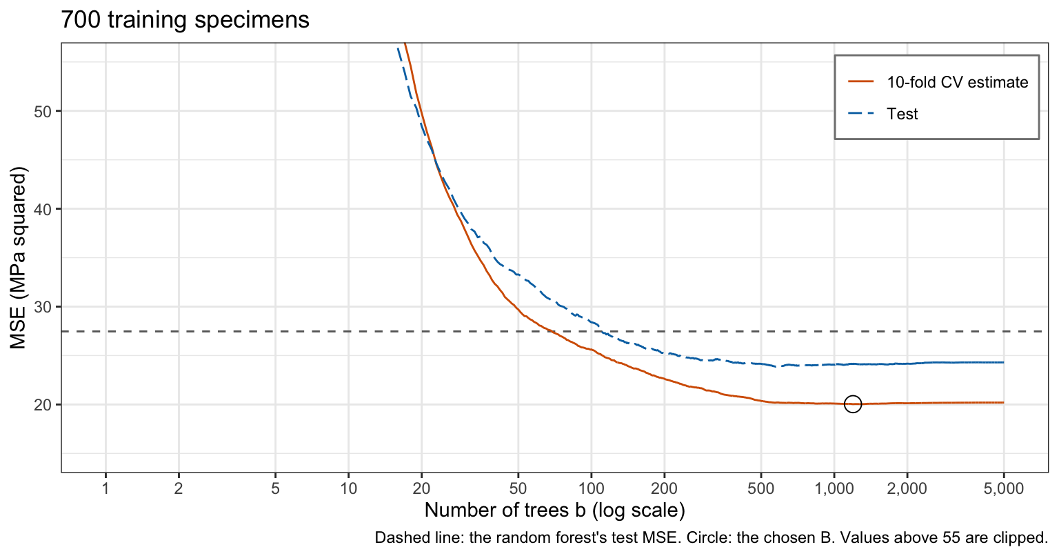
The cross-validation estimate is smallest, 20.0, at \(B = 1{,}194\). The chosen model, with \(\nu = 0.1\), \(\delta = 4\) and \(B = 1{,}194\), is refit to all the training specimens:
# The chosen model: B_cv trees, fit to all the training specimens.
fit_cv <- xgb.train(params, d_train, nrounds = B_cv)
mean((y_test - predict(fit_cv, d_test))^2)
[1] 24.14392Its test MSE is 24.1; the smallest test MSE over every number of trees, which cross-validation cannot know, is 23.9, after 573 trees. The estimate is within 1% of its minimum for every \(B\) from 546 to 5,000, so \(B = 1{,}194\) is not sharply determined; minimizing \(\overline{\text{RMSE}}(B)\) alone would choose \(B = 1{,}312\).
The cross-validation estimate is below the test MSE by 4.1. This lecture does not fully explain the gap. Cross-validation reports the minimum of a noisy curve, and the test MSE comes from one sample of 305 specimens. Repeated mixes do not explain it by themselves: 72% of the training specimens share their mix with a training specimen in another fold, and 68% of the test specimens have a mix that some training specimen also has.
29.5 Variable importance
29.5.1 RSS decrease
A boosted model of hundreds of trees has no single tree to read. Its variable importance summarizes which explanatory variables its splits use, and how much those splits improve the fit.
A split of a node of a tree fit to residuals decreases their RSS by \[\frac{n_1 n_2}{n_1 + n_2}\left(\bar r_1 - \bar r_2\right)^2,\] where
- \(n_1\) and \(n_2\) are the numbers of training specimens in the two parts of the node, and
- \(\bar r_1\) and \(\bar r_2\) are their mean residuals.
This is the decrease of the Decision Trees lecture with the residuals as the response. The importance of explanatory variable \(X_j\) is the sum of these decreases over every split on \(X_j\) in all \(B\) trees, usually reported as a share of the total over the \(p\) variables.
xgboost calls a split’s decrease its gain: \[\text{gain} = \frac{S_1^2}{n_1 + \texttt{lambda}} + \frac{S_2^2}{n_2 + \texttt{lambda}} - \frac{S^2}{n_1 + n_2 + \texttt{lambda}},\] where
- \(S_1\) and \(S_2\) are the sums of the residuals in the two parts,
- \(S = S_1 + S_2\) is the sum over the node, and
lambdais the leaf penalty of the Loop reproduction subsection.
With lambda = 0, \(S_k^2/n_k = n_k\bar r_k^2\), and the gain is \(n_1\bar r_1^2 + n_2\bar r_2^2 - (n_1 + n_2)\bar r^2\), with \(\bar r\) the mean residual of the node, which equals the decrease in RSS above. With the default lambda = 1 each denominator is one larger, a small change for nodes of many specimens. xgb.importance() returns one row per explanatory variable; its Gain column is the variable’s total gain over all splits and trees, divided by the total over all variables, so the column sums to 1. For the chosen model:
# Each variable's share of the total gain of the chosen model's splits.
importance_boost <- xgb.importance(fit_cv)
importance_boost[, c("Feature", "Gain")]
Feature Gain
<char> <num>
1: age 0.36214097
2: cement 0.29837558
3: superplasticizer 0.08909573
4: water 0.08908287
5: blast_furnace_slag 0.06942685
6: fine_aggregate 0.05293820
7: fly_ash 0.01997255
8: coarse_aggregate 0.01896725
NoteCode
# With lambda = 0, the gains of the loop-settings fit are its decreases in
# RSS: their total over all splits equals the total decrease in RSS of the
# loop's trees (rpart()'s variable.importance, without surrogate splits).
loop_total_gain <- sum(xgb.model.dt.tree(loop_fit) |>
                         filter(Feature != "Leaf") |>
                         pull(Gain))
loop_decrease <- sum(unlist(map(trees, "variable.importance")))
stopifnot(abs(loop_total_gain / loop_decrease - 1) < 1e-3)

# The shares of the chosen model, by variable.
boost_share <- set_names(importance_boost$Gain, importance_boost$Feature)
top_boost <- names(boost_share)[1:2]
The other two columns, Cover and Frequency, measure how many training specimens pass through a variable’s splits and how many splits use it; this lecture uses Gain. age and cement carry 66% of the chosen model’s total gain.
29.5.2 Forest and tree importance
The same decrease in RSS measures the importance of a variable in a single tree, summed over its splits, and in a random forest, summed over the splits of each tree and averaged over the trees (randomForest() reports it as IncNodePurity; the Random Forests lecture has a second measure).
NoteCode
# Decrease in RSS by explanatory variable as a share of the total, for the
# chosen boosted model, the random forest, and the pruned tree.
share_of <- function(x) {
  x / sum(x)
}

# Random forest: IncNodePurity, the decrease in RSS averaged over trees.
forest_share <- share_of(importance(best_rf)[, "IncNodePurity"])

# Pruned tree: the decrease in RSS of each split, read from the RSS of
# each node and of its two children in the frame (rpart()'s own
# variable.importance would include surrogate splits).
tree_decrease <- function(fit) {
  frame <- fit$frame
  nodes <- as.integer(rownames(frame))
  internal <- frame$var != "<leaf>"
  parent <- nodes[internal]
  decrease <- frame$dev[internal] -
    frame$dev[match(2 * parent, nodes)] -
    frame$dev[match(2 * parent + 1, nodes)]
  tapply(decrease, as.character(frame$var[internal]), sum)
}
tree_share <- share_of(tree_decrease(all_pruned))

# One row per method and variable; a variable a fit never splits on has
# share 0.
method_names <- c("Boosting",
                  paste0("Random forest, m = ", m_best),
                  "Pruned tree")
shares <- list(boost_share, forest_share, tree_share)
importance_long <- map2(shares, method_names, \(share, method) {
  tibble(method = method, variable = explanatory,
         share = coalesce(as.numeric(share[explanatory]), 0))
}) |>
  list_rbind() |>
  mutate(method = factor(method, levels = method_names))

# Variables in the order of the boosting shares.
boost_rank <- names(sort(boost_share, decreasing = TRUE))
forest_rank <- names(sort(forest_share, decreasing = TRUE))
tree_rank <- names(sort(tree_share, decreasing = TRUE))
importance_long <- importance_long |>
  mutate(variable = factor(variable, levels = rev(boost_rank)))

# Share: major lines every 10%, minor lines midway.
share_top <- ceiling(max(importance_long$share) / 0.1) * 0.1
importance_plot <- ggplot(importance_long, aes(x = share, y = variable)) +
  geom_segment(aes(x = 0, xend = share, yend = variable), color = "grey60") +
  geom_point(size = 2.5) +
  facet_wrap(~ method) +
  scale_x_continuous(breaks = seq(0, share_top, by = 0.1),
                     minor_breaks = seq(0.05, share_top, by = 0.1),
                     limits = c(0, share_top),
                     labels = scales::label_percent()) +
  labs(x = "Share of the total decrease in RSS", y = NULL,
       title = title_train)

# The top two variables of each method and, if they are the same two, the
# share of each method's decrease in RSS that they carry, for prose.
top_two <- list(boost_rank[1:2], forest_rank[1:2], tree_rank[1:2])
same_top_two <- all(map_lgl(top_two, \(x) setequal(x, top_two[[1]])))
top_text <- if (same_top_two) {
  top_vars <- top_two[[1]]
  top_shares <- map_dbl(shares, \(share) sum(share[top_vars]))
  paste0("All three put ", and_list(code(sort(top_vars))),
         " in the first two places, with ", pct(top_shares[1], 0),
         " of the boosted model's decrease in RSS, ",
         pct(top_shares[2], 0), " of the forest's, and ",
         pct(top_shares[3], 0), " of the tree's; below them the orders ",
         "differ.")
} else {
  "The three fits do not agree on the first two places."
}

# The prose says the orders below the first two places differ.
below_two <- map(list(boost_rank, forest_rank, tree_rank), \(x) x[-(1:2)])
stopifnot(!all(map_lgl(below_two, \(x) identical(x, below_two[[1]]))))
The figure plots the shares for the boosted model of the chosen 1,194 trees (Gain), for the random forest with \(m = 5\), and for the pruned tree of the Decision Trees lecture, the variables in the order of the boosting shares.
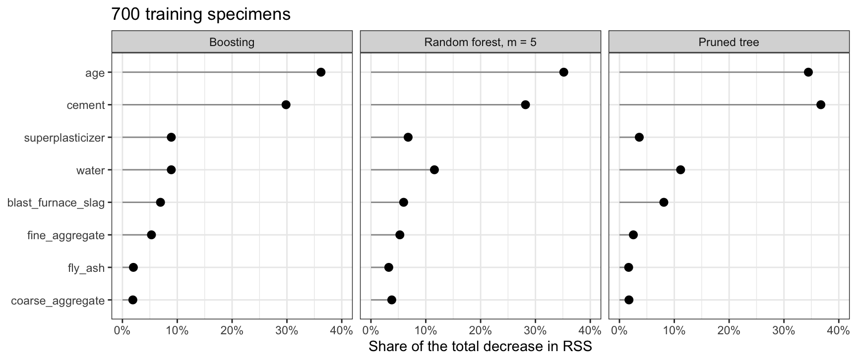
Boosting ranks the variables age, cement, superplasticizer, water, blast_furnace_slag, fine_aggregate, fly_ash, and coarse_aggregate; the random forest ranks them age, cement, water, superplasticizer, blast_furnace_slag, fine_aggregate, coarse_aggregate, and fly_ash; the pruned tree ranks them cement, age, water, blast_furnace_slag, superplasticizer, fine_aggregate, coarse_aggregate, and fly_ash. All three put age and cement in the first two places, with 66% of the boosted model’s decrease in RSS, 63% of the forest’s, and 71% of the tree’s; below them the orders differ.
29.5.3 Interpretation
Importance ranks the variables; it gives no direction and no effect size. A large share for age says that the trees’ splits on age decrease the RSS by a large total, not whether concrete gets stronger or weaker with age, with the other ingredients fixed, or by how much. The Additive structure section shows what the model predicts as age changes.
29.6 Additive structure
29.6.1 Cement and age
Does the effect of cement on strength depend on age?
NoteCode
# Training specimens in the lowest and the highest third of cement content.
cement_cuts <- quantile(train$cement, c(1 / 3, 2 / 3))
third_names <- paste(c("Cement at most", "Cement at least"),
                     fmt(cement_cuts, 0), "kg per cubic meter")
thirds <- train |>
  mutate(age_jit = age_jit,
         third = case_when(cement <= cement_cuts[[1]] ~ third_names[1],
                           cement >= cement_cuts[[2]] ~ third_names[2])) |>
  filter(!is.na(third)) |>
  mutate(third = factor(third, levels = third_names))

# Mean strength of each third at each age with at least min_per_age
# specimens in both thirds, and the gap between the two means.
min_per_age <- 5
third_means <- thirds |>
  summarise(strength = mean(compressive_strength), n = n(),
            .by = c(third, age)) |>
  filter(n >= min_per_age) |>
  filter(n_distinct(third) == 2, .by = age)
third_gaps <- third_means |>
  pivot_wider(id_cols = age, names_from = third, values_from = strength) |>
  mutate(gap = .data[[third_names[2]]] - .data[[third_names[1]]])
gap_low <- slice_min(third_gaps, gap, n = 1, with_ties = FALSE)
gap_max <- max(third_gaps$gap)
gap_max_ages <- sort(third_gaps$age[third_gaps$gap >= gap_max - 0.1])

# The prose says the high-cement third is stronger at every such age.
stopifnot(all(third_gaps$gap > 0))

# How the thirds differ in the other six ingredients: the difference of
# their means in training standard deviations, and the two largest.
other_ingredients <- setdiff(ingredients, "cement")
ingredient_gaps <- map_dbl(other_ingredients, \(v) {
  high <- mean(thirds[[v]][thirds$third == third_names[2]])
  low <- mean(thirds[[v]][thirds$third == third_names[1]])
  (high - low) / sd(train[[v]])
}) |>
  set_names(other_ingredients)
top_ingredients <- names(sort(abs(ingredient_gaps), decreasing = TRUE))[1:2]
top_names <- str_replace_all(top_ingredients, "_", " ")
top_signs <- sign(ingredient_gaps[top_ingredients])
ingredient_text <- if (all(top_signs < 0)) {
  paste0("chiefly ", and_list(top_names),
         ", of which the high-cement third has less")
} else if (all(top_signs > 0)) {
  paste0("chiefly ", and_list(top_names),
         ", of which the high-cement third has more")
} else {
  paste0("chiefly ", top_names[1], " (",
         if (top_signs[1] > 0) "more" else "less", " in the high-cement ",
         "third) and ", top_names[2], " (",
         if (top_signs[2] > 0) "more" else "less", ")")
}

# Strength against age, by third, with the means joined by lines.
third_plot <- ggplot(thirds, aes(x = age_jit, y = compressive_strength,
                                 color = third, shape = third,
                                 linetype = third)) +
  geom_point(alpha = 0.35, size = 1) +
  geom_line(data = third_means, aes(x = age, y = strength),
            linewidth = 0.9) +
  geom_point(data = third_means, aes(x = age, y = strength), size = 2.5) +
  scale_color_manual(values = okabe_ito[c(1, 5)]) +
  age_axis +
  scale_y_continuous(breaks = seq(0, 80, by = 20),
                     minor_breaks = seq(10, 90, by = 20),
                     limits = c(0, 90)) +
  labs(x = "Age (days, log scale)", y = "Compressive strength (MPa)",
       color = NULL, shape = NULL, linetype = NULL,
       title = paste(nrow(thirds), "training specimens")) +
  theme(legend.position = "inside",
        legend.position.inside = c(0.01, 0.97),
        legend.justification = c(0, 1),
        legend.background = element_rect(color = "grey50"))
The figure plots the strength of the training specimens in the lowest and the highest third of cement content against age, with the mean strength of each third at every age with at least 5 specimens in both thirds.
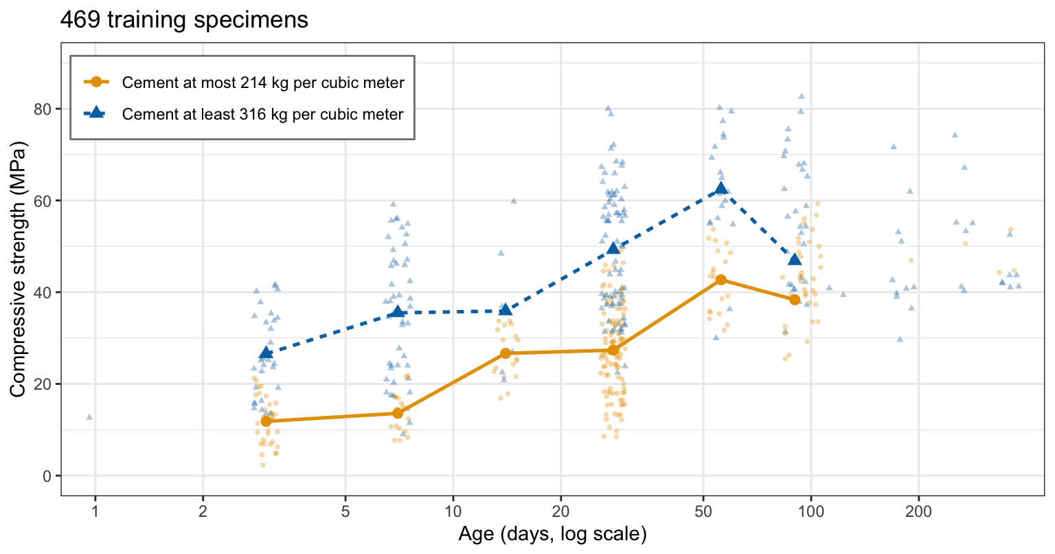
The high-cement third is stronger at every such age, by 8.5 MPa at 90 days and by about 22 MPa at 7 and 28 days. The two thirds also differ in other ingredients, chiefly fly ash and blast furnace slag, of which the high-cement third has less, so this raw comparison does not isolate cement; a model can.
29.6.2 Stumps
The figure above asks whether the gap in strength between high- and low-cement mixes changes with age. A boosted model of stumps cannot let it change. A stump depends on one explanatory variable. Collecting the stumps that split on each variable, a boosted model of stumps is a sum of functions, each of which depends on one variable,
\[\hat f_B(x) = \sum_{j=1}^p a_j(x), \qquad a_j(x) = \sum_{b:\, \hat f^b \text{ splits on } X_j} \nu\,\hat f^b(x),\]
where \(a_j(x)\) is the sum of the shrunken stumps that split on \(X_j\), which depends on \(x\) only through the value of \(X_j\). (xgboost’s start at the mean strength adds a constant, which belongs to no variable and changes no difference.)
This is an additive model: the change in the prediction when the value of \(X_j\) changes does not depend on the values of the other variables.
NoteCode
# A grid: age from 1 to 365 days, two cement contents, the other
# ingredients at their training medians.
cement_levels <- c(200, 400)
medians <- summarise(train, across(all_of(ingredients), median))
age_grid <- exp(seq(log(1), log(365), length.out = 300))
grid <- expand_grid(age = age_grid, cement = cement_levels) |>
  bind_cols(select(medians, -cement)) |>
  select(all_of(explanatory))

# Predictions on the grid from the stumps (all B_max trees) and from the
# chosen model of depth 4.
stump_fit <- depth_runs[[which(depth_values == 1)]]$fit
grid_fits <- list(Stumps = predict(stump_fit, grid),
                  `Depth 4` = predict(fit_cv, grid))
grid_curves <- map2(grid_fits, names(grid_fits), \(fit, model) {
  mutate(grid, strength = fit, model = model)
}) |>
  list_rbind()

# The gap between the two cement contents at each age, for each model.
gaps <- grid_curves |>
  pivot_wider(id_cols = c(model, age), names_from = cement,
              values_from = strength) |>
  mutate(gap = .data[[as.character(cement_levels[2])]] -
           .data[[as.character(cement_levels[1])]]) |>
  summarise(low = min(gap), high = max(gap), .by = model)
gap_of <- function(model_name, column) {
  filter(gaps, model == model_name)[[column]]
}

# The prose says the stumps' gap is the same at every age (xgboost
# predicts in single precision, hence the tolerance).
stopifnot(gap_of("Stumps", "high") - gap_of("Stumps", "low") < 1e-3)

# Predicted strength against age, one line per cement content; the
# models' tabs share their axes.
cement_names <- paste(cement_levels, "kg of cement per cubic meter")
strength_axis <- scale_y_continuous(breaks = seq(0, 80, by = 20),
                                    minor_breaks = seq(-10, 90, by = 20),
                                    limits = c(-10, 90))
additive_plot <- function(model_name) {
  curves <- grid_curves |>
    filter(model == model_name) |>
    mutate(cement = factor(cement, levels = cement_levels,
                           labels = cement_names))
  ggplot(curves, aes(x = age, y = strength, color = cement,
                     linetype = cement)) +
    geom_line(linewidth = 0.9) +
    scale_color_manual(values = okabe_ito[c(1, 5)]) +
    age_axis +
    strength_axis +
    labs(x = "Age (days, log scale)", y = "Predicted strength (MPa)",
         color = NULL, linetype = NULL,
         title = "Other ingredients at their training medians") +
    theme(legend.position = "inside",
          legend.position.inside = c(0.99, 0.03),
          legend.justification = c(1, 0),
          legend.background = element_rect(color = "grey50"))
}
additive_plots <- map(names(grid_fits), additive_plot)
additive_plots <- do.call(patchwork::align_patches, additive_plots)

# Number of explanatory variables each tree of the chosen depth-4 model
# splits on, from the table of its splits.
vars_per_tree <- xgb.model.dt.tree(fit_cv) |>
  filter(Feature != "Leaf") |>
  summarise(n_vars = n_distinct(Feature), .by = Tree) |>
  pull(n_vars)
stopifnot(length(vars_per_tree) == B_cv)

# The smallest test MSE of each depth above 1, for prose.
interaction_depths <- depth_values[-1]
interaction_text <- and_list(paste(fmt(map_dbl(interaction_depths,
                                               depth_at), 1),
                                   "for depth", interaction_depths))
A tree of depth \(\delta\) can split on more than \(\delta\) explanatory variables in all: the 1,194 trees of depth 4 of the chosen model split on 2 to 8, with median 5. But each leaf is reached through at most \(\delta\) splits, so the tree’s prediction is a sum, over its leaves, of a constant times an indicator that involves at most \(\delta\) variables. A boosted model of such trees is a sum of such terms, so it can represent interactions among at most \(\delta\) variables.
The tabs plot the predicted strength against age for mixes with 200 and 400 kg of cement per cubic meter, the other six ingredients at their medians among the training specimens: first for the boosted model of 5,000 stumps with \(\nu = 0.1\), then for the chosen model of 1,194 trees of depth 4.
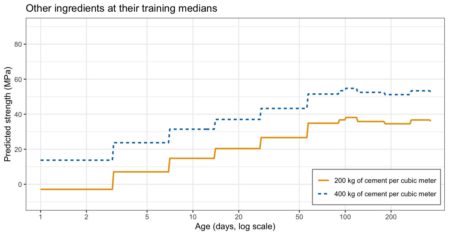
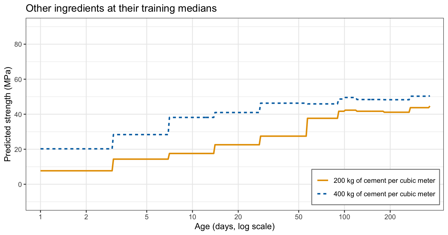
For the stumps the two curves are parallel: the extra cement adds 16.6 MPa to the prediction at every age. For the trees of depth 4, the gap runs from 5.9 to 20.6 MPa, depending on age: the effect of cement on strength depends on age, an interaction, as the raw thirds suggested.
Whether the interactions matter is a question for the test error. In the Tree depth figure, the stumps’ test MSE after 5,000 trees, 31.7 and still falling slowly, is above the smallest test MSE of every depth that allows interactions: 28.1 for depth 2, 23.9 for depth 4, and 28.2 for depth 8.
29.7 Comparison
29.7.1 Bias and variance
NoteCode
# Bagging with small trees: trees of depth 1 and of depth 4, each grown as
# far as the depth allows on a bootstrap sample of the training specimens;
# the test MSE of the average of the first b trees.
n_bagged <- 1000
small_depths <- c(1, 4)
bag_small <- map(small_depths, \(d) {
  control <- depth_control(d)
  pred <- sapply(seq_len(n_bagged), \(b) {
    boot <- sample(n_train, replace = TRUE)
    tree <- rpart(compressive_strength ~ ., data = train[boot, ],
                  control = control)
    predict(tree, test)
  })
  running <- t(apply(pred, 1, cumsum)) /
    matrix(seq_len(n_bagged), nrow(test), n_bagged, byrow = TRUE)
  tibble(depth = d, trees = seq_len(n_bagged),
         test = colMeans((y_test - running)^2), method = "Bagging")
}) |>
  list_rbind()

# Boosting with the same depths, from the Tree depth fits.
boost_small <- filter(depth_curves, depth %in% small_depths) |>
  select(depth, trees, test) |>
  mutate(method = "Boosting")

# Test MSE of one tree of each depth fit to all the training specimens.
single_small <- map_dbl(small_depths, \(d) {
  tree <- rpart(compressive_strength ~ ., data = train,
                control = depth_control(d))
  mse(y_test, predict(tree, test))
}) |>
  set_names(small_depths)

# Test MSE of each method with all its trees.
small_end <- bind_rows(bag_small, boost_small) |>
  slice_max(trees, n = 1, by = c(method, depth))
end_of <- function(method_name, d) {
  filter(small_end, method == method_name, depth == d)$test
}

# Test MSE against the number of trees, one panel per depth.
depth_names <- paste("Trees of depth", small_depths)
small_curves <- bind_rows(bag_small, boost_small) |>
  mutate(depth = factor(depth, levels = small_depths, labels = depth_names))
small_ylim <- c(0, 200)

# Number of trees on a log scale, for the narrower panels: powers of 10,
# minor lines midway in log space.
decade_axis <- scale_x_log10(breaks = 10^(0:3),
                             minor_breaks = 10^(seq(0.5, 3.5, by = 1)),
                             labels = scales::label_comma())
small_plot <- ggplot(small_curves, aes(x = trees, y = test, color = method,
                                       linetype = method)) +
  geom_line() +
  facet_wrap(~ depth) +
  scale_color_manual(values = okabe_ito[c(5, 4)]) +
  decade_axis +
  scale_y_continuous(breaks = seq(0, 200, by = 50),
                     minor_breaks = seq(25, 175, by = 50)) +
  coord_cartesian(ylim = small_ylim) +
  labs(x = "Number of trees b (log scale)", y = "Test MSE (MPa squared)",
       color = NULL, linetype = NULL, title = title_train,
       caption = paste0("Bagging: ", big(n_bagged), " trees; boosting: ",
                        big(B_max), ". Values above ", small_ylim[2],
                        " are clipped.")) +
  theme(legend.position = "bottom")

# The prose says boosting ends below bagging at both depths, and bagging
# below the single tree.
stopifnot(end_of("Boosting", 1) < end_of("Bagging", 1),
          end_of("Boosting", 4) < end_of("Bagging", 4),
          end_of("Bagging", 1) < single_small[["1"]],
          end_of("Bagging", 4) < single_small[["4"]])
The figure plots the test MSE against the number of trees for bagging and for boosting (\(\nu = 0.1\)) with the same small trees, stumps and trees of depth 4.
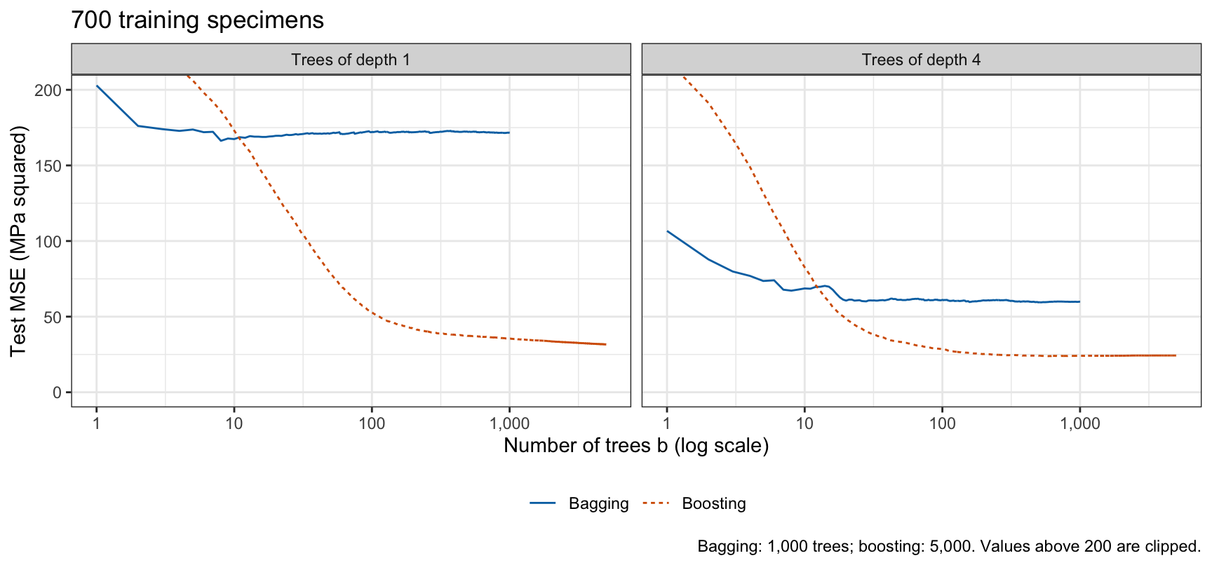
One stump fit to all the training specimens has test MSE 183.6, and one tree of depth 4 92.9. Averaging 1,000 of them over bootstrap samples brings these to 171.7 and 59.9; boosting trees of the same depths brings them to 31.7 and 24.3 with 5,000 trees. A small tree’s error is mostly bias: it cannot follow the curve in age, or the effect of the other ingredients, with a few leaves. Averaging removes variance but leaves the bias of the trees it averages, so bagging needs large trees. Boosting removes bias: each tree is fit to what the trees before it got wrong, so the sum of many small trees can follow a function no single small tree can.
29.7.2 Test error
NoteCode
# The pruned tree's 10-fold CV estimate of its MSE, at the cp that defines
# it. rpart()'s xerror is the CV sum of squared errors divided by the root
# node's RSS (the frame's first dev), so xerror times the root node's MSE,
# the training MSE of the mean prediction, is the CV MSE.
root_mse <- all_full$frame$dev[1] / n_train
stopifnot(abs(root_mse - mse(y_train, mean(y_train))) < 1e-8)
pruned_row <- which.min(all_cp[, "xerror"])
stopifnot(all_cp[pruned_row, "CP"] == all_best_cp)
pruned_cv <- all_cp[pruned_row, "xerror"] * root_mse
# The conversion checked on fixed folds, which draw no random numbers: the
# MSE of xpred.rpart()'s out-of-fold predictions equals xerror times the
# root node's MSE at every cp.
check_folds <- rep_len(1:10, n_train)
check_control <- rpart.control(cp = 0, minsplit = 2, minbucket = 1,
xval = check_folds)
check_tree <- rpart(compressive_strength ~ ., data = train,
control = check_control)
check_pred <- xpred.rpart(check_tree, xval = check_folds)
check_cv <- colMeans((y_train - check_pred)^2)
check_xerror <- check_tree$cptable[, "xerror"] * root_mse
stopifnot(max(abs(check_cv - check_xerror)) < 1e-8)
# The OOB MSE after the last tree of the bagging forest and of the forest
# with the OOB choice of m (m_oob), and boosting's CV estimate at B_cv.
estimate_mse <- c(pruned = pruned_cv,
bagging = m_oob[[p]],
forest = m_oob[[m_best]],
boosting = cv_best)
# Test MSE of every fit on all eight explanatory variables, how each was
# tuned, and its CV or OOB estimate where it has one.
comparison <- tribble(
~Method, ~Tuning, ~estimate, ~value,
"Least squares, main effects", "none", NA, earlier_mse[["ls"]],
"Least squares with log(age)", "none", NA, earlier_mse[["log_ls"]],
"Default tree", "rpart() stopping rules", NA, earlier_mse[["default"]],
"Full tree", "none", NA, earlier_mse[["full"]],
"Pruned tree", "cp by 10-fold CV", estimate_mse[["pruned"]],
earlier_mse[["pruned"]],
paste0("Bagging, $m = ", p, "$"), "none", estimate_mse[["bagging"]],
forest_mse[["bagging"]],
paste0("Random forest, $m = ", m_best, "$"), "$m$ by OOB error",
estimate_mse[["forest"]], forest_mse[["forest"]],
paste0("Boosting, $\\nu = ", nu_main, "$, $\\delta = ", depth_main, "$"),
paste0("$\\nu$ and $\\delta$ fixed in advance, $B = ", big_math(B_cv),
"$ by 10-fold CV"), estimate_mse[["boosting"]], boost_mse
)
# An en dash (as an HTML entity) where a fit has no CV or OOB estimate.
comparison <- comparison |>
mutate(estimate = if_else(is.na(estimate), "–", fmt(estimate, 1)),
value = fmt(value, 1))
comparison_table <- knitr::kable(comparison,
col.names = c("Method", "Tuning",
"CV/OOB MSE", "Test MSE"),
align = "llrr")
# Each CV/OOB MSE minus the test MSE of the same fit, for prose: the
# direction and size of the gaps, stated as one pattern when all four go
# the same way.
fit_test_mse <- c(pruned = earlier_mse[["pruned"]],
bagging = forest_mse[["bagging"]],
forest = forest_mse[["forest"]],
boosting = boost_mse)
estimate_gap <- estimate_mse - fit_test_mse
fit_names <- c(pruned = "the pruned tree",
bagging = "bagging",
forest = "the random forest",
boosting = "boosting")
gap_side <- if_else(estimate_gap > 0, "above", "below")
gap_by <- paste0(fit_names, " (by ", fmt(abs(estimate_gap), 1), ")")
gap_text <- if (all(gap_side == gap_side[1])) {
paste0("The CV/OOB MSE is ", gap_side[1], " the test MSE of the same ",
"fit for ", and_list(gap_by), ".")
} else {
paste0("The CV/OOB MSE is above the test MSE of the same fit for ",
and_list(gap_by[gap_side == "above"]), ", and below it for ",
and_list(gap_by[gap_side == "below"]), ".")
}
# Boosting's test MSE relative to the best of the other fits.
others_best <- min(earlier_mse, forest_mse)
others_best_name <- if (others_best == forest_mse[["forest"]]) {
"the random forest"
} else if (others_best == forest_mse[["bagging"]]) {
"bagging"
} else {
"the best of the other fits"
}
boost_gain <- 1 - boost_mse / others_best
best_text <- if (boost_mse < others_best) {
paste0("Boosting has the smallest test MSE, ", fmt(boost_mse, 1), ", ",
pct(boost_gain, 0), " below ", others_best_name, "'s ",
fmt(others_best, 1), ".")
} else {
paste0("Boosting's test MSE, ", fmt(boost_mse, 1), ", is not the ",
"smallest; ", others_best_name, " has ", fmt(others_best, 1),
".")
}
# The smallest test MSE of boosting at each other depth, over B, for the
# prose comparison with the forest.
other_depths <- setdiff(depth_values, depth_main)
other_depth_mse <- map_dbl(other_depths, depth_at)
n_below <- sum(other_depth_mse < others_best)
other_text <- if (n_below == length(other_depths)) {
"all below"
} else if (n_below == 0) {
"all above"
} else {
paste(n_below, "of them below")
}
# The depth with the smallest test MSE in the Tree depth figure, a
# comparison on the test specimens that chose nothing.
depth_text <- paste0("In the Tree depth figure, a comparison on the test ",
"specimens, $\\delta = ", best_depth, "$ has the ",
"smallest test MSE of the depths compared; that ",
"comparison illustrates the depth and did not ",
"choose it.")
# Noise the chapter shows in test MSE: the two implementations of the same
# algorithm, and the refit forests against the previous lecture's.
implementation_gap <- abs(mse(y_test, loop_fit_test) - loop_test)The table collects the test MSE of every fit to all 8 explanatory variables in the three tree lectures, with how each was tuned and its cross-validation or OOB estimate of the test MSE (CV/OOB MSE): for the pruned tree, rpart()’s 10-fold CV estimate at the chosen cp, for bagging and the random forest the OOB MSE, and for boosting \(\text{CV}_{(10)}(B)\) at the chosen \(B\). Least squares, the default tree and the full tree have no such estimate here.
| Method | Tuning | CV/OOB MSE | Test MSE |
|---|---|---|---|
| Least squares, main effects | none | – | 106.4 |
| Least squares with log(age) | none | – | 48.5 |
| Default tree | rpart() stopping rules | – | 86.8 |
| Full tree | none | – | 40.3 |
| Pruned tree | cp by 10-fold CV | 60.8 | 42.2 |
| Bagging, \(m = 8\) | none | 27.3 | 26.9 |
| Random forest, \(m = 5\) | \(m\) by OOB error | 26.8 | 27.5 |
| Boosting, \(\nu = 0.1\), \(\delta = 4\) | \(\nu\) and \(\delta\) fixed in advance, \(B = 1{,}194\) by 10-fold CV | 20.0 | 24.1 |
The CV/OOB MSE is above the test MSE of the same fit for the pruned tree (by 18.5) and bagging (by 0.4), and below it for the random forest (by 0.6) and boosting (by 4.1). A CV/OOB MSE and a test MSE differ by noise, since they are computed on different specimens, and by selection: at the tuning it chose, an estimate is the smallest value it found.
Boosting has the smallest test MSE, 24.1, 10% below bagging’s 26.9. Differences of a few units of test MSE are within the noise this chapter shows: the loop and xgboost with the loop’s settings, the same algorithm, differ by 1.3, the refit forests differ from the previous lecture’s by up to 0.8, and every test MSE comes from one sample of 305 test specimens. For boosting, \(\nu = 0.1\) and \(\delta = 4\) were fixed in advance and only \(B\) was chosen, by cross-validation. In the Tree depth figure, a comparison on the test specimens, \(\delta = 4\) has the smallest test MSE of the depths compared; that comparison illustrates the depth and did not choose it. Taking the best \(B\) for each other depth, chosen on the test specimens and so flattering to boosting, depths 1, 2, and 8 reach 31.6, 28.1, and 28.2, all above bagging’s 26.9: boosting’s advantage depends on its tuning parameters. Least squares with \(\log(\texttt{age})\), which needed a feature built after seeing the curve in age, has 48.5; the tree ensembles find the curve and any interactions without it.
29.7.3 Limits
Boosting has three tuning parameters, \(B\), \(\nu\), and \(\delta\), against a random forest’s \(m\) and number of trees, and xgboost adds more, such as lambda. Its \(B\) must be chosen, since too many trees overfit, while a forest only needs enough trees. Its trees are grown in sequence, each needing the residuals of the one before, so they cannot be grown at the same time as a forest’s can (xgboost instead spreads the split search of each tree over processor threads), and the cross-validation above grew 5,000 trees in each of 10 folds. With many trees it fits the training data nearly exactly: the training MSE fell to 0.28 with \(\nu = 0.5\), while that fit’s test MSE never fell below 21.0. Like a forest, it has no single tree to read, only importance rankings, its predictions are made of steps, and it predicts a constant beyond the largest value of an explanatory variable in the training data, since every tree does.
NoteBeyond this course
- Tuning every parameter. \(\nu\) and \(\delta\) can be chosen by cross-validation along with \(B\), running
xgb.cv()for each pair of values on a grid, andlambdaandmin_child_weightcan be tuned the same way; this lecture does not. - Classification. Gradient boosting for a class fits each tree to the negative gradient of the deviance of a logistic or multinomial model in place of the residuals; the boosted model predicts the log-odds. In
xgboostthis isobjective = "binary:logistic"or"multi:softprob". AdaBoost, an early boosting method, instead reweights the observations, giving more weight at each step to those the trees so far misclassify. - Other packages. The ISLR2 lab fits boosted trees with
gbm::gbm(), whosen.trees,shrinkageandinteraction.depthare \(B\), \(\nu\) and \(\delta\), and which starts from the mean of the response. LightGBM and CatBoost are other widely used implementations of gradient boosting. - Bayesian additive regression trees. BART (ISLR2 Section 8.2.4) also fits a sum of trees to residuals, but changes each tree a little at a time by random perturbations and averages over many such sums.
29.8 Conclusion
Boosting builds a model from small trees added one after another. It starts from a constant fit, fits a tree of depth \(\delta\) to the current residuals, adds \(\nu\) times the tree’s predictions to the fit, and updates the residuals, \(B\) times. Each tree is fit to what the trees before it got wrong, so the trees depend on one another and are grown in sequence. The algorithm is a short loop of rpart() fits; xgboost implements it, with \(\nu\), \(\delta\) and \(B\) as learning_rate, max_depth and nrounds, and by default starts from the mean response and shrinks each leaf’s prediction with the penalty lambda.
The three tuning parameters interact. The shrinkage \(\nu\) sets how fast the model learns: a smaller \(\nu\) needs more trees and makes the test error less sensitive to their number. The depth \(\delta\) sets how complex each tree is: each leaf of a tree of depth \(\delta\) is reached through at most \(\delta\) splits, so the boosted model is a sum of terms that each involve at most \(\delta\) explanatory variables and can represent interactions among at most \(\delta\) of them. Stumps give an additive model, a sum of functions that each depend on one variable. The number of trees \(B\) is a tuning parameter like \(\nu\) and \(\delta\); unlike them here, it is chosen without the test data by cross-validation, and it must be chosen, since, unlike bagging, boosting overfits when \(B\) is too large. One run of boosting per fold, as in xgb.cv(), gives the cross-validation estimate for every \(B\) up to its length.
Bagging and random forests average large trees, each with low bias and high variance, grown independently on bootstrap samples, which reduces variance. Boosting adds small trees, each with high bias, fit to residuals, which reduces bias. The importance of an explanatory variable, the decrease in RSS from its splits summed over the trees (xgboost’s gain), ranks the variables without giving a direction or an effect size.
The next lecture begins support vector machines (ISLR2 Chapter 9), which classify by finding a boundary that separates the classes in the space of the features, with as wide a margin as possible.