# All rows, and the explanatory variables.
concrete <- modeldata::concrete
n_rows <- nrow(concrete)
explanatory <- setdiff(names(concrete), "compressive_strength")
p <- length(explanatory)

# Rows that repeat an earlier row exactly, and rows that repeat the mix and
# age of an earlier row with a different strength.
n_exact <- sum(duplicated(concrete))
n_same_mix <- sum(duplicated(select(concrete, all_of(explanatory))))
n_replicate <- n_same_mix - n_exact

# One row per specimen.
specimens <- distinct(concrete)
n_specimens <- nrow(specimens)

# The ages at which specimens were tested.
ages <- sort(unique(specimens$age))27 Decision Trees
TipLearning objectives
After this lecture you should be able to
- describe a regression tree as a partition of the values of the explanatory variables into regions \(R_1, \ldots, R_L\), with the mean training response of a region as the prediction for every observation in it, and read a prediction from a fitted tree’s printout or diagram,
- derive the best single split, the explanatory variable \(j\) and cut point \(s\) that minimize the summed RSS of the two regions, show that the decrease in RSS is \(n_1n_2\left(\bar y_1 - \bar y_2\right)^2/\left(n_1 + n_2\right)\), and explain why recursive binary splitting is greedy and top-down,
- explain cost-complexity pruning, the criterion \(\text{RSS} + \alpha|T|\) and its nested sequence of subtrees, choose \(\alpha\) by 10-fold cross-validation, and evaluate the pruned tree on test data,
- compute the classification error rate, the Gini index, and the entropy of a node and of a split, and explain why the Gini index or the entropy, not the error rate, is used to grow a classification tree,
- fit regression and classification trees with
rpart(), prune them withprune(), and evaluate them by test MSE or by a test confusion matrix, and - compare trees with linear models: interpretability, nonlinearity and interactions without feature engineering, predictions that are piecewise constant, and high variance.
Most models so far have been linear in a set of features, with any curvature or interaction built into the features by hand. A decision tree instead splits the values of the explanatory variables into rectangles and predicts a constant in each. It needs no features built by hand: each split is on one explanatory variable as recorded. This lecture grows trees for a numeric response (regression trees) and for a class (classification trees), and prunes them back. The reading is ISLR2 Section 8.1.
27.1 Concrete strength
27.1.1 Data
Question. How well do the ingredients of a concrete mix and its age predict how much load the concrete can bear?
Data. modeldata::concrete records laboratory tests of concrete cylinders (Yeh 2006, “Analysis of Strength of Concrete Using Design of Experiments and Neural Networks,” Journal of Materials in Civil Engineering 18). Each observation is a specimen: one cylinder of one mix, crushed at one age. The response is the compressive strength, compressive_strength, in megapascals (MPa). The explanatory variables are the amounts of seven ingredients, in kg per cubic meter of mix, and the age of the specimen in days.
NoteCode
The 1,030 rows include 25 that repeat an earlier row exactly, strength included. These are treated as duplicated records of one specimen, and distinct() removes them so that no specimen is both a training and a test specimen. Another 13 rows repeat the mix and age of an earlier row with a different strength; they are separate specimens and stay. That leaves 1,005 specimens, tested at 14 ages from 1 to 365 days.
27.1.2 Training specimens
# The training sample size.
n_train <- 700

# Training specimens: a random sample; every other specimen is a test
# specimen.
train_id <- sample(n_specimens, n_train)
train <- specimens[train_id, ]
test <- specimens[-train_id, ]
The split leaves 700 training specimens and 305 test specimens. The figure plots the strength of each training specimen against its age, on a log scale, and against its cement content.
NoteCode
# Ages repeat, so each training specimen's age is jittered once, by up to
# 8% either way, and the jittered age is used in every figure.
jitter_factor <- 0.08
train_plot <- train |>
  mutate(age_jit = age * exp(runif(n(), -jitter_factor, jitter_factor)))

# Age on a log scale: major lines at 1, 2, 5, 10, 20, 50, 100 and 200 days,
# no minor lines; the limits run past the youngest and oldest specimens.
age_limits <- c(0.8, 450)
age_axis <- scale_x_log10(breaks = c(1, 2, 5, 10, 20, 50, 100, 200),
                          minor_breaks = NULL,
                          limits = age_limits,
                          expand = expansion(0))

# Cement: major lines every 100 kg per cubic meter, minor lines midway.
cement_limits <- c(100, 550)
cement_axis <- scale_x_continuous(breaks = seq(100, 500, by = 100),
                                  minor_breaks = seq(150, 550, by = 100),
                                  limits = cement_limits,
                                  expand = expansion(0))

# Strength: major lines every 20 MPa, minor lines midway.
strength_axis <- scale_y_continuous(breaks = seq(0, 80, by = 20),
                                    minor_breaks = seq(10, 90, by = 20),
                                    limits = c(0, 90))

# Strength against age and against cement, side by side.
title_train <- paste(n_train, "training specimens")
strength_age <- ggplot(train_plot,
                       aes(x = age_jit, y = compressive_strength)) +
  geom_point(alpha = 0.4, size = 1) +
  age_axis +
  strength_axis +
  labs(x = "Age (days, log scale)", y = "Compressive strength (MPa)")
strength_cement <- ggplot(train, aes(x = cement,
                                     y = compressive_strength)) +
  geom_point(alpha = 0.4, size = 1) +
  cement_axis +
  strength_axis +
  labs(x = "Cement (kg per cubic meter)", y = NULL)
data_plot <- patchwork::wrap_plots(strength_age, strength_cement) +
  patchwork::plot_annotation(title = title_train)

# Mean strength at 3 and at 28 days, and the share of specimens at 28 days.
age_means <- train |>
  summarise(strength = mean(compressive_strength), .by = age)
mean_at <- function(a) {
  age_means$strength[age_means$age == a]
}
share_28 <- mean(train$age == 28)

# Share of the test specimens whose mix, the seven ingredients, is the mix
# of some training specimen.
ingredients <- setdiff(explanatory, "age")
train_mixes <- distinct(select(train, all_of(ingredients)))
mix_seen <- semi_join(test, train_mixes, by = ingredients)
share_mix_seen <- nrow(mix_seen) / nrow(test)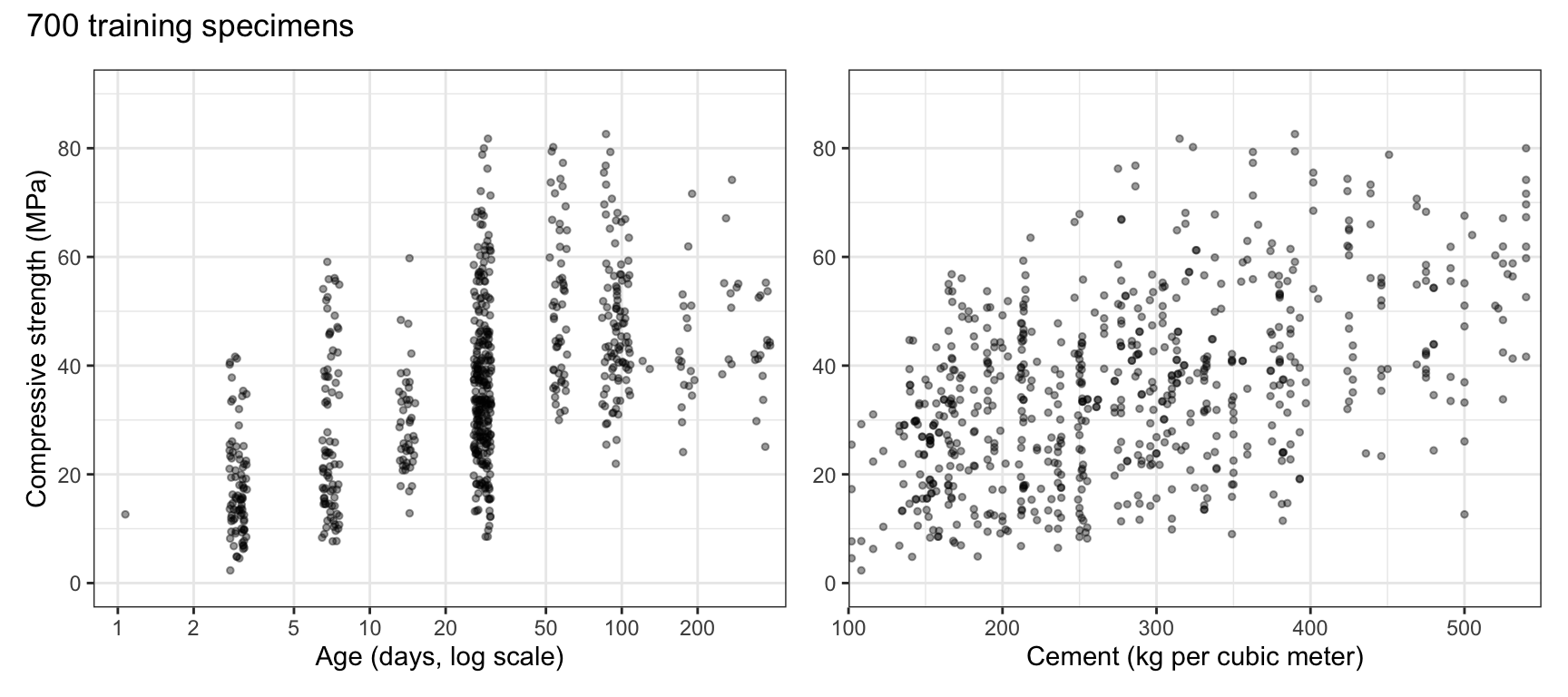
Strength rises steeply with age over the first month, from a mean of 17.6 MPa at 3 days to 36.6 MPa at 28 days, and more slowly, and noisily, afterward; 40% of the training specimens were tested at 28 days, the standard age for testing concrete. Strength rises with cement too, with a wide spread at every cement content: specimens with the same cement differ in age and in the other six ingredients. The relation with age is far from a straight line, and a linear model would need features, such as a log of age, built for that curvature.
Many mixes were tested at several ages: 68% of the test specimens have a mix, the seven ingredients, that some training specimen also has. The test MSEs below therefore measure predictions for mixes like those tested, often at a new age, not for mixes never tested.
27.2 Regression trees
27.2.1 Age and cement
The figure plots the training specimens by their age and their cement content, with color showing strength.
NoteCode
# Cement on the vertical axis, with the same limits and grid lines.
cement_y_axis <- scale_y_continuous(breaks = seq(100, 500, by = 100),
                                    minor_breaks = seq(150, 550, by = 100),
                                    limits = cement_limits,
                                    expand = expansion(0))

# Strength as color, on the viridis scale, which also runs from dark to
# light; legend marks every 20 MPa.
strength_color <- scale_color_viridis_c(breaks = seq(0, 80, by = 20),
                                        limits = c(0, 90))
plane_plot <- ggplot(train_plot, aes(x = age_jit, y = cement,
                                     color = compressive_strength)) +
  geom_point(size = 1.5) +
  strength_color +
  age_axis +
  cement_y_axis +
  labs(x = "Age (days, log scale)", y = "Cement (kg per cubic meter)",
       color = "Strength\n(MPa)", title = title_train)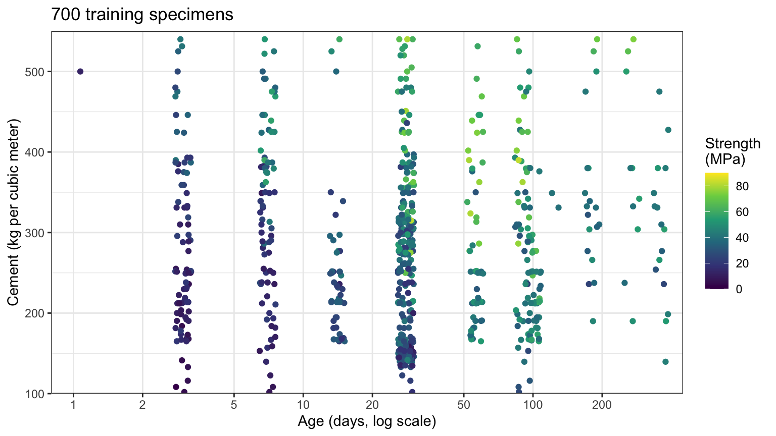
The dark, weak specimens sit at the left, at young ages, and in the bottom band of low cement; the light, strong ones sit at the right and the top. A vertical line near 3 weeks and a horizontal line or two in cement would already separate much of the weak concrete from the strong.
27.2.2 Regions and predictions
A regression tree turns those lines into a model. It divides the values of the explanatory variables into \(L\) non-overlapping rectangles, the regions \(R_1, \ldots, R_L\), and predicts the mean training response of a region for every observation that falls in it:
\[\hat f(x) = \sum_{\ell=1}^{L} \hat y_{R_\ell}\,\mathrm{I}\left(x \in R_\ell\right),\]
where
- \(x\) is a value of the \(p\) explanatory variables \(X = (X_1, \ldots, X_p)\),
- \(R_\ell\) is the \(\ell\)th region, a rectangle in the \(p\) explanatory variables,
- \(\hat y_{R_\ell}\) is the mean response of the training observations in \(R_\ell\), and
- \(\mathrm{I}\left(x \in R_\ell\right)\) is 1 if \(x\) falls in \(R_\ell\) and 0 otherwise.
A tree splits on the explanatory variables as recorded, so in this chapter each feature is an explanatory variable. Observation \(i\) has values \(x_i = (x_{i1}, \ldots, x_{ip})\), with \(x_{ij}\) the value of explanatory variable \(X_j\), and response \(y_i\).
For given regions, the tree’s training RSS is
\[\text{RSS} = \sum_{\ell=1}^{L}\sum_{i:\, x_i \in R_\ell}\left(y_i - \hat y_{R_\ell}\right)^2.\]
Within one region, \(\sum_{i:\, x_i \in R_\ell}\left(y_i - c\right)^2\) has derivative \(-2\sum_{i:\, x_i \in R_\ell}\left(y_i - c\right)\) in \(c\), which is zero at the region’s mean, so the mean is the constant with the smallest RSS in that region. The regions themselves are harder: there are too many ways to partition the values into rectangles to search them all, so a tree builds its regions one split at a time.
27.2.3 Best split
A split of a region \(R\) on explanatory variable \(j\) at cut point \(s\) makes two regions,
\[R_1(j, s) = \left\{X \in R \mid X_j < s\right\}, \qquad R_2(j, s) = \left\{X \in R \mid X_j \ge s\right\},\]
where
- \(R\) is the region being split (at the first split, every value of the explanatory variables),
- \(X_j\) is explanatory variable \(j\), and
- \(s\) is the cut point.
The best split is the pair \((j, s)\) that minimizes
\[\sum_{i:\, x_i \in R_1(j, s)}\left(y_i - \hat y_{R_1}\right)^2 + \sum_{i:\, x_i \in R_2(j, s)}\left(y_i - \hat y_{R_2}\right)^2,\]
the RSS of the two regions after the split.
Write \(n_1\) and \(n_2\) for the numbers of training observations in the two regions, \(\bar y_1 = \hat y_{R_1}\) and \(\bar y_2 = \hat y_{R_2}\) for their means, \(n_R = n_1 + n_2\) for the number in the region being split (the training sample size \(n\) only at the first split), and \(\bar y = \left(n_1\bar y_1 + n_2\bar y_2\right)/n_R\) for the mean before the split. In \(R_1\), \(\sum\left(y_i - \bar y\right)^2 = \sum\left(y_i - \bar y_1\right)^2 + n_1\left(\bar y_1 - \bar y\right)^2\), because the cross term \(2\left(\bar y_1 - \bar y\right)\sum\left(y_i - \bar y_1\right)\) is zero, and likewise in \(R_2\). Since \(\bar y_1 - \bar y = n_2\left(\bar y_1 - \bar y_2\right)/n_R\) and \(\bar y_2 - \bar y = -n_1\left(\bar y_1 - \bar y_2\right)/n_R\), the RSS before the split minus the RSS after it is
\[n_1\left(\bar y_1 - \bar y\right)^2 + n_2\left(\bar y_2 - \bar y\right)^2 = \frac{n_1 n_2}{n_1 + n_2}\left(\bar y_1 - \bar y_2\right)^2.\]
The best split separates two means as far apart as possible, weighted toward regions of similar size. The RSS after the split changes only when \(s\) crosses an observed value of \(X_j\), so only the cut points between consecutive distinct values need checking: at most \(n_R - 1\) for each explanatory variable. rpart() uses the midpoints.
NoteCode
# Decrease in RSS, as a share of the RSS before the split, for every cut
# point of explanatory variable v: the midpoints of its distinct values.
split_curve <- function(data, v, y = "compressive_strength") {
  values <- sort(unique(data[[v]]))
  cuts <- (head(values, -1) + tail(values, -1)) / 2
  response <- data[[y]]
  rss_before <- sum((response - mean(response))^2)
  decrease <- map_dbl(cuts, \(s) {
    left <- data[[v]] < s
    n_1 <- sum(left)
    n_2 <- sum(!left)
    gap <- mean(response[left]) - mean(response[!left])
    n_1 * n_2 / (n_1 + n_2) * gap^2
  })
  tibble(variable = v, cut = cuts, share = decrease / rss_before)
}

# Every cut point of every explanatory variable at the root, and the best
# cut point of each explanatory variable.
root_curves <- map(explanatory, \(v) split_curve(train, v)) |>
  list_rbind()
root_best <- root_curves |>
  slice_max(share, n = 1, with_ties = FALSE, by = variable) |>
  arrange(desc(share))
best_age <- filter(root_best, variable == "age")
best_cement <- filter(root_best, variable == "cement")

# Share of the RSS removed: major lines every 10%, minor lines midway.
share_axis <- scale_y_continuous(breaks = seq(0, 0.4, by = 0.1),
                                 minor_breaks = seq(0.05, 0.35, by = 0.1),
                                 limits = c(0, 0.35),
                                 labels = scales::label_percent())

# The curves for age and cement, the best cut point of each circled.
curve_panel <- function(v) {
  curve <- filter(root_curves, variable == v)
  best <- filter(root_best, variable == v)
  ggplot(curve, aes(x = cut, y = share)) +
    geom_line() +
    geom_point(size = 1) +
    geom_point(data = best, size = 4, shape = 1) +
    share_axis
}
age_curve <- curve_panel("age") +
  age_axis +
  labs(x = "Cut point s on age (days, log scale)",
       y = "Share of RSS removed")
cement_curve <- curve_panel("cement") +
  cement_axis +
  labs(x = "Cut point s on cement (kg per cubic meter)", y = NULL)
curve_plot <- patchwork::wrap_plots(age_curve, cement_curve) +
  patchwork::plot_annotation(title = title_train,
                             caption = "Circles: the best cut point.")
The figure plots, for every cut point \(s\) on age and on cement, the share of the training RSS that the split of all 700 training specimens removes.
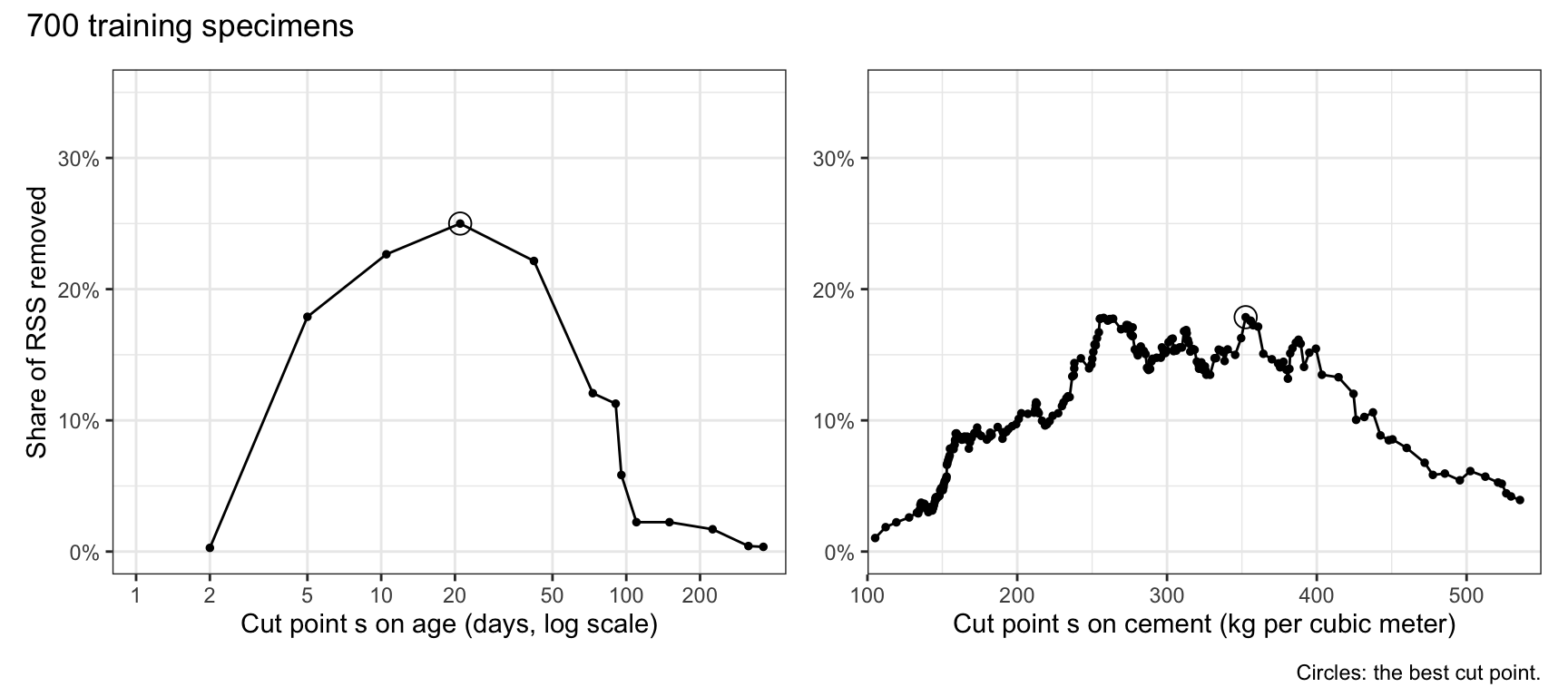
The best split on age is at \(s = 21\) days, which removes 25.0% of the RSS; the best split on cement is at \(s = 352.5\) kg per cubic meter, which removes 17.9%. With specimens tested at only 14 ages, age has only 13 cut points to check. Over all 8 explanatory variables, the best first split is on age, with cement next (17.9%).
27.2.4 Recursive binary splitting
A tree repeats the best split inside each region it creates:
- Start with all the training observations in one region, the root.
- In each current region, find the best split \((j, s)\) of the training observations in that region alone, and split.
- Repeat in each new region until a stopping rule holds.
The search is greedy: each split is the best one at its own step, chosen without looking ahead to the splits it makes possible later. It is top-down: it starts from the root and works down. The regions at the end are the leaves, or terminal nodes; the splits are the internal nodes.
rpart() stops splitting a region when it holds fewer than 20 training observations, when a split would leave a leaf with fewer than 7, or when the best split would lower the tree’s RSS by less than 1% of the RSS of the root, the default complexity parameter cp. These are defaults, chosen for speed; the Pruning section that follows chooses the tree’s size from the data instead. The tree rpart() grows with these defaults is called the default tree below.
27.2.5 Fitting
# The default tree on age and cement.
two_fit <- rpart(compressive_strength ~ age + cement, data = train)
two_fit
n= 700
node), split, n, deviance, yval
* denotes terminal node
1) root 700 188853.400 35.76574
2) age< 21 219 35098.050 23.59484
4) cement< 354.5 156 11805.220 18.54385
8) age< 10.5 113 4471.562 15.02124 *
9) age>=10.5 43 2246.643 27.80093 *
5) cement>=354.5 63 9457.747 36.10206
10) age< 5 24 1784.060 28.62667 *
11) age>=5 39 5507.202 40.70231 *
3) age>=21 481 106544.400 41.30717
6) cement< 352.5 378 61539.100 37.40508
12) cement< 164.8 81 6032.791 25.56395 *
13) cement>=164.8 297 41051.690 40.63448
26) age< 42 156 20125.900 36.77500
52) cement< 257.7 62 6430.345 32.35226 *
53) cement>=257.7 94 11682.890 39.69213 *
27) age>=42 141 16031.170 44.90454 *
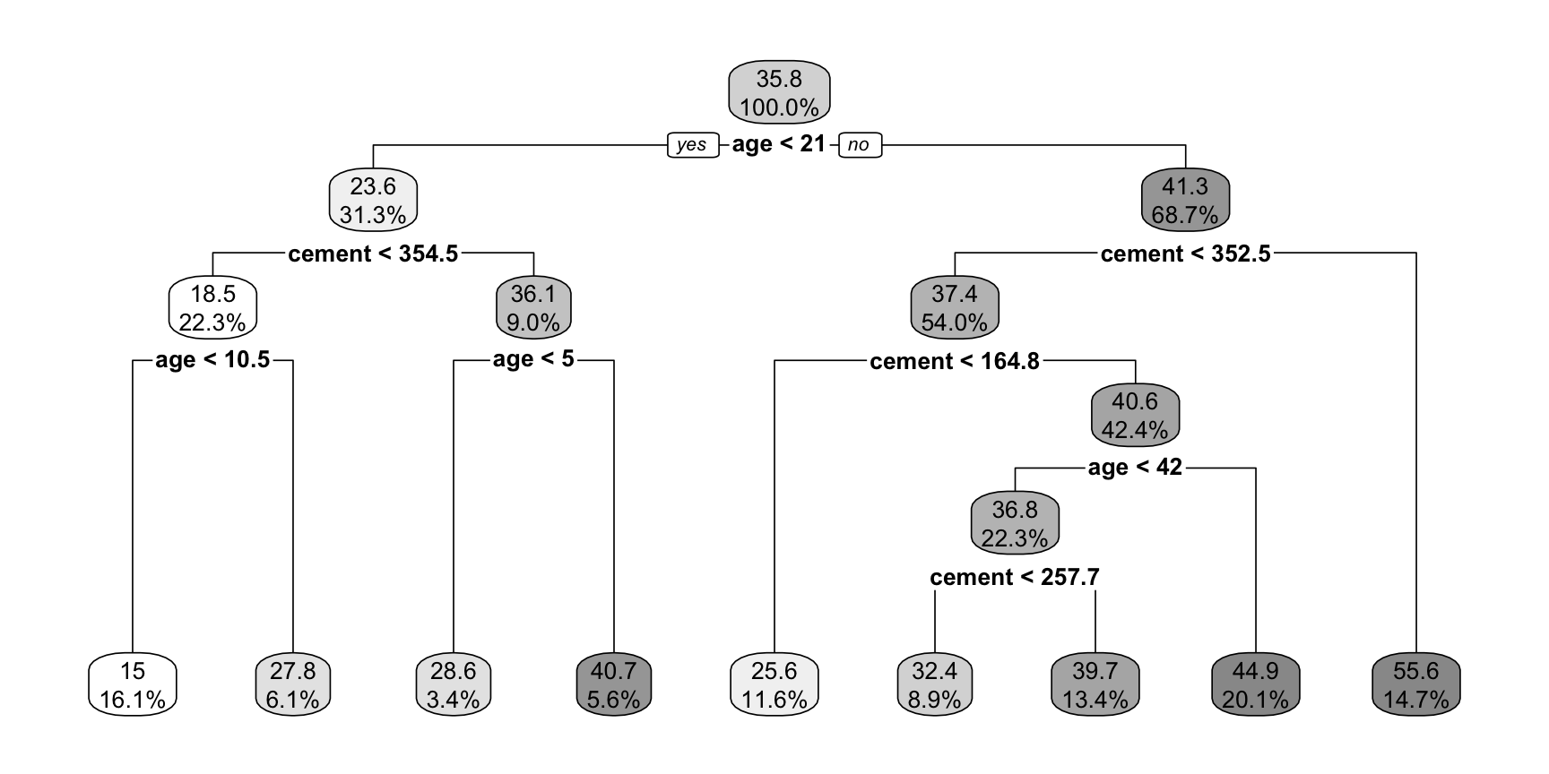
7) cement>=352.5 103 18127.390 55.62748 *Each line is a node: its number, the split that leads to it, its number of training specimens, its RSS (deviance), and its mean strength (yval). An asterisk marks a leaf. Node 1, the root, holds all 700 specimens, with mean 35.8 MPa. The first split sends the specimens younger than 21 days to node 2 and the rest to node 3, and each node \(m\) has children \(2m\) and \(2m + 1\). A specimen’s prediction is the mean of the leaf it reaches. The tree has 9 leaves.
NoteCode
# The variable and cut point of each internal node: the primary split of
# each internal node comes first in its block of rows of fit$splits.
node_splits <- function(fit) {
  frame <- fit$frame
  internal <- frame$var != "<leaf>"
  block <- 1 + frame$ncompete[internal] + frame$nsurrogate[internal]
  first_row <- cumsum(c(1, head(block, -1)))
  tibble(node = as.integer(rownames(frame)[internal]),
         variable = as.character(frame$var[internal]),
         cut = fit$splits[first_row, "index"])
}

# Split labels with exact cut points: rpart.plot() otherwise rounds them to
# the digits of the node values.
exact_labels <- function(fit) {
  # rpart.plot() labels each node with the split that leads to it, the
  # split of its parent, node %/% 2; the root has none.
  splits <- node_splits(fit)
  nodes <- as.integer(rownames(fit$frame))
  parent_cut <- splits$cut[match(nodes %/% 2, splits$node)]
  function(x, labs, digits, varlen, faclen) {
    exact <- str_replace(labs, "[0-9.]+$", as.character(parent_cut))
    if_else(is.na(parent_cut), labs, exact)
  }
}

# Draw a tree: each node shows its mean (or class) and its share of the
# training observations; splits are written below the nodes.
draw_tree <- function(fit, box.palette = "Grays", ...) {
  rpart.plot(fit, type = 2, roundint = FALSE, box.palette = box.palette,
             split.fun = exact_labels(fit), ...)
}
The diagram draws the same tree. Each box shows a node’s mean strength and its share of the training specimens; a specimen goes left when the condition under the box holds.
NoteFor example,
A specimen of 28 days with 300 kg of cement per cubic meter is at least 21 days old, so it goes right at the root; from there it follows the cement and age conditions down to a leaf. Its prediction is 39.7 MPa, the mean strength of the training specimens in that leaf.
27.2.6 Partition
The tabs draw the tree’s regions over the training specimens, one level of splits at a time; the last tab is the whole fitted tree. Each rectangle is a leaf, labeled with its mean strength.
NoteCode
# The rectangle of each leaf of a tree on two explanatory variables, from
# the conditions on the path to the leaf, within the given limits.
leaf_rectangles <- function(fit, limits) {
  is_leaf <- fit$frame$var == "<leaf>"
  leaves <- as.integer(rownames(fit$frame)[is_leaf])
  paths <- path.rpart(fit, nodes = leaves, print.it = FALSE)
  rectangles <- map(paths, \(conditions) {
    bounds <- limits
    for (condition in conditions[-1]) {
      parts <- str_match(condition, "^(\\w+)\\s*(<|>=)\\s*(.+)$")
      v <- parts[2]
      s <- as.numeric(parts[4])
      if (parts[3] == "<") {
        bounds[[v]][2] <- min(bounds[[v]][2], s)
      } else {
        bounds[[v]][1] <- max(bounds[[v]][1], s)
      }
    }
    tibble(xmin = bounds[[1]][1], xmax = bounds[[1]][2],
           ymin = bounds[[2]][1], ymax = bounds[[2]][2])
  })
  list_rbind(rectangles) |>
    mutate(node = leaves, value = fit$frame$yval[is_leaf])
}

# The tree cut back to its first `depth` levels of splits: node m is at
# depth floor(log2(m)), and the internal nodes at `depth` become leaves.
first_levels <- function(fit, depth) {
  nodes <- as.integer(rownames(fit$frame))
  internal <- fit$frame$var != "<leaf>"
  toss <- nodes[internal & floor(log2(nodes)) == depth]
  if (length(toss) == 0) {
    return(fit)
  }
  snip.rpart(fit, toss = toss)
}

# Regions of a tree on age and cement, shaded and labeled by their means,
# over the specimens it was fit to.
concrete_limits <- list(age = age_limits, cement = cement_limits)
strength_fill <- scale_fill_viridis_c(limits = c(0, 90), guide = "none")
partition_plot <- function(fit, label_size = 3.5, data = train_plot,
                           title = title_train, min_height = 0) {
  rectangles <- leaf_rectangles(fit, concrete_limits) |>
    mutate(x = sqrt(xmin * xmax), y = (ymin + ymax) / 2)

  # Regions too thin for a label, in kg per cubic meter, go unlabeled.
  labeled <- filter(rectangles, ymax - ymin >= min_height)
  ggplot() +
    geom_rect(data = rectangles,
              aes(xmin = xmin, xmax = xmax, ymin = ymin, ymax = ymax,
                  fill = value),
              alpha = 0.5, color = "black") +
    geom_point(data = data, aes(x = age_jit, y = cement),
               size = 0.6, alpha = 0.5) +
    geom_label(data = labeled,
               aes(x = x, y = y, label = fmt(value, 1)),
               size = label_size, linewidth = 0, alpha = 0.8) +
    strength_fill +
    age_axis +
    cement_y_axis +
    labs(x = "Age (days, log scale)", y = "Cement (kg per cubic meter)",
         title = title)
}

# One plot per level of splits of the default tree.
two_depth <- max(floor(log2(as.integer(rownames(two_fit$frame)))))
level_plots <- map(seq_len(two_depth), \(d) {
  partition_plot(first_levels(two_fit, d))
})

# The tabs name five levels, the last the fitted tree; line up their panels.
stopifnot(two_depth == 5)
level_plots <- do.call(patchwork::align_patches, level_plots)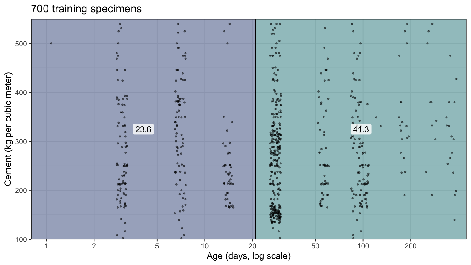
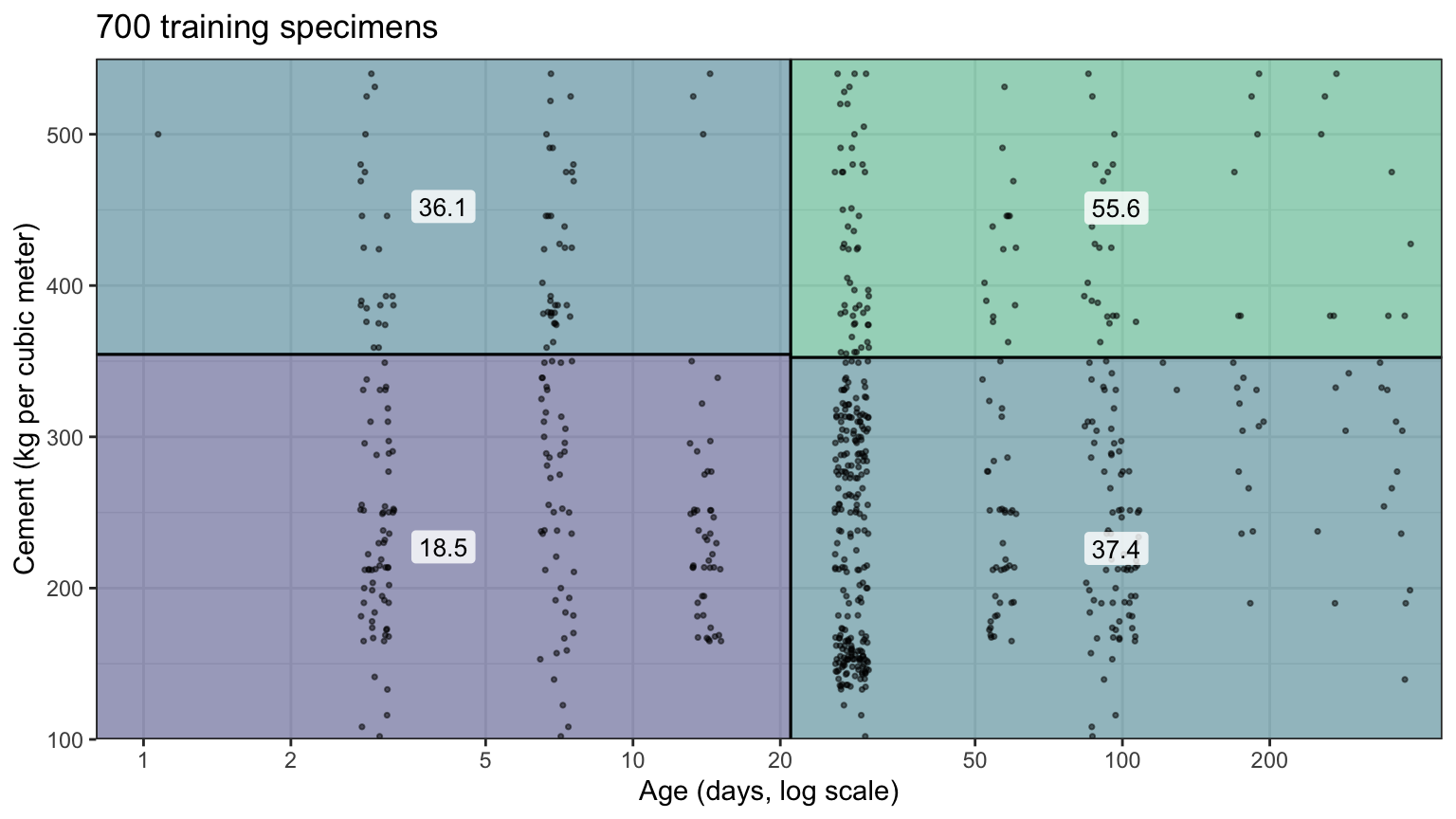
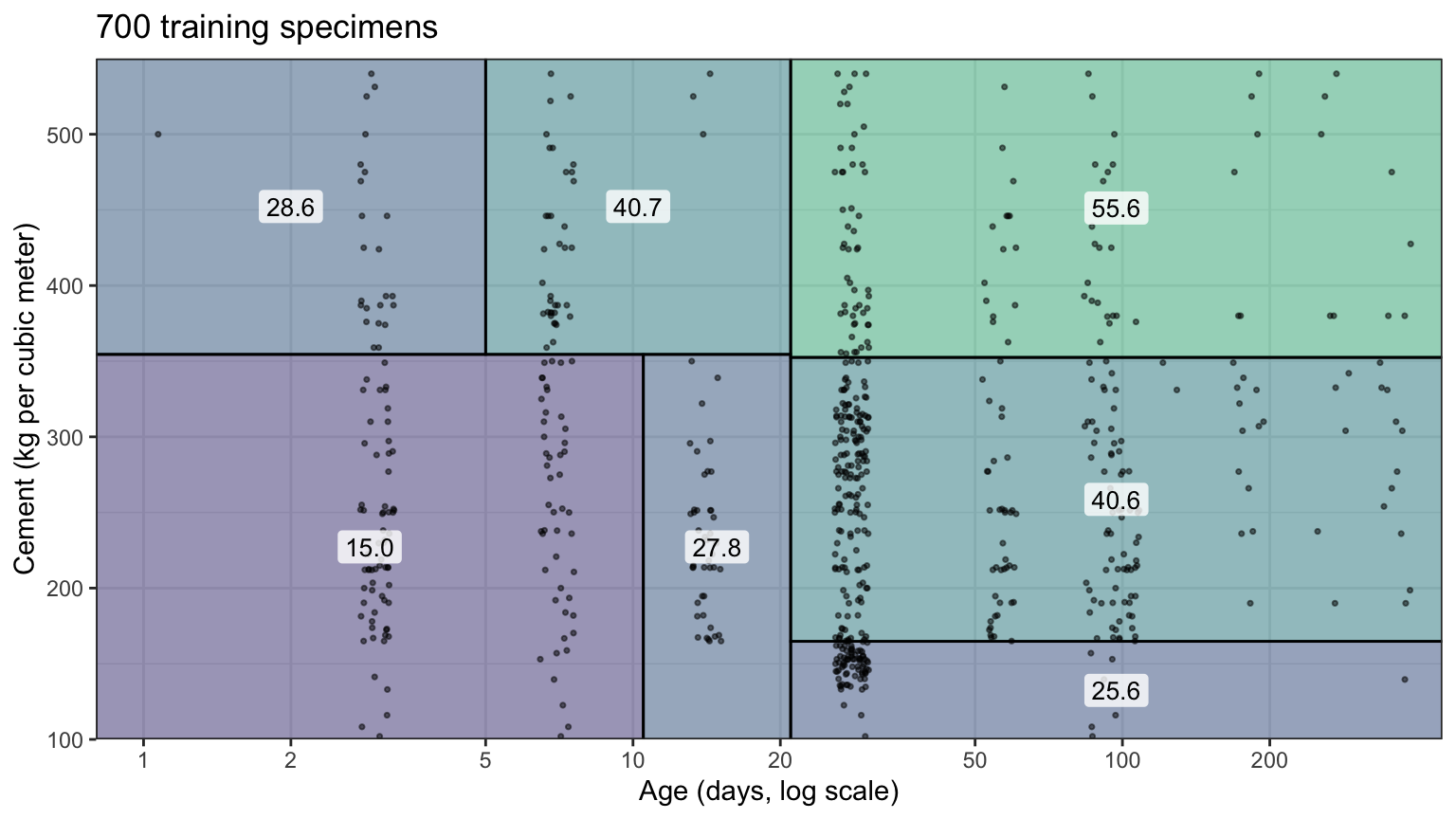
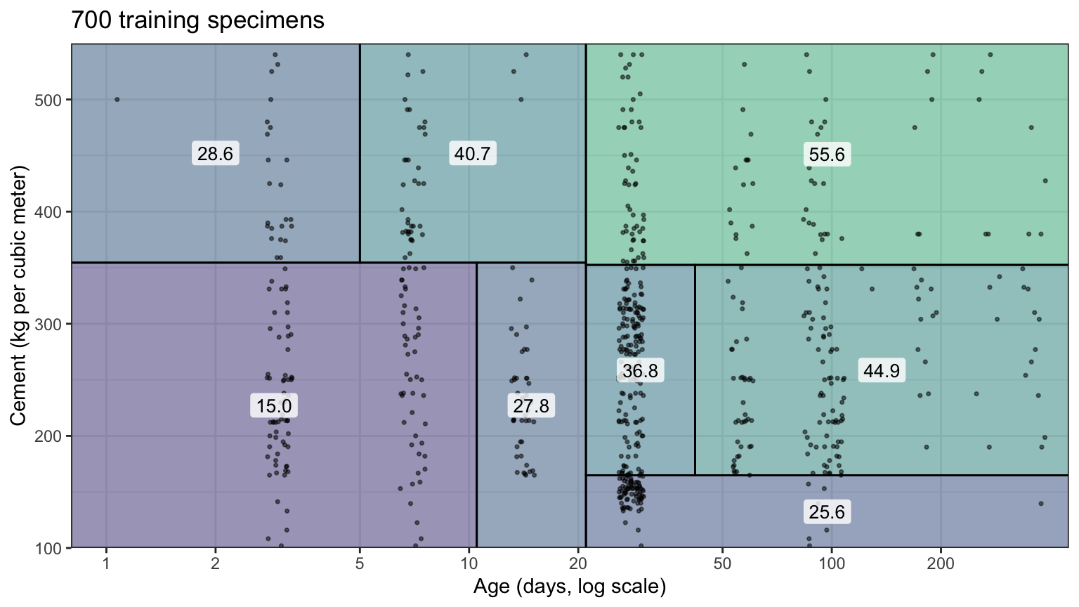
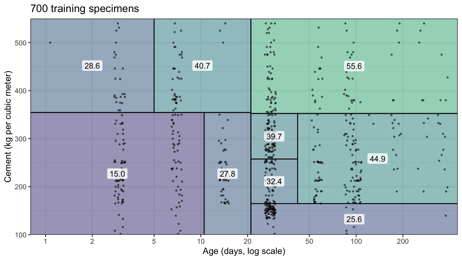
The fitted tree has 5 levels of splits, so its tab is the fifth level. Every boundary is a vertical or horizontal line, and each later split divides only the region it is made in: after the first split on age, the young and the old specimens are split on cement at different cut points. The fitted function is a step function in two explanatory variables, constant on each rectangle and jumping at its edges.
27.3 Pruning
27.3.1 Overfitting
This section prunes the tree on age and cement only. With all 8 explanatory variables the full tree’s test MSE is no worse than the pruned tree’s, as the All explanatory variables subsection below shows.
The default stopping rules ended the tree at 9 leaves. Growing it without them, until no region can be split, gives the full tree \(T_0\).
# The full tree: no threshold on the decrease in RSS, and leaves as small
# as one specimen.
full_control <- rpart.control(cp = 0, minsplit = 2, minbucket = 1)
full_fit <- rpart(compressive_strength ~ age + cement, data = train,
                  control = full_control)

# Number of leaves.
c(leaves = sum(full_fit$frame$var == "<leaf>"))
leaves
564
NoteCode
# The cross-validation table of the full tree, one row per subtree.
cp_table <- full_fit$cptable

# Training and test MSE of every subtree in the table.
y_train <- train$compressive_strength
y_test <- test$compressive_strength
size_curve <- map(seq_len(nrow(cp_table)), \(k) {
  subtree <- prune(full_fit, cp = cp_table[k, "CP"])
  tibble(leaves = cp_table[k, "nsplit"] + 1,
         Training = mse(y_train, predict(subtree, train)),
         Test = mse(y_test, predict(subtree, test)))
}) |>
  list_rbind()

# The subtree with the smallest test MSE, and the full tree.
test_best <- slice_min(size_curve, Test, n = 1, with_ties = FALSE)
full_row <- slice_tail(size_curve, n = 1)

# Number of leaves on a log scale: major lines at 1, 2, 5, 10, ..., 500, no
# minor lines.
leaves_axis <- scale_x_log10(breaks = c(1, 2, 5, 10, 20, 50, 100, 200, 500),
                             minor_breaks = NULL)

# MSE: major lines every 50, minor lines midway.
mse_axis <- scale_y_continuous(breaks = seq(0, 300, by = 50),
                               minor_breaks = seq(25, 325, by = 50),
                               limits = c(0, 300))
mse_labels <- c("Training", "Test")
size_long <- size_curve |>
  pivot_longer(-leaves, names_to = "data", values_to = "mse") |>
  mutate(data = factor(data, levels = mse_labels))
size_plot <- ggplot(size_long, aes(x = leaves, y = mse, color = data,
                                   linetype = data)) +
  geom_line() +
  scale_color_manual(values = okabe_ito[c(5, 4)]) +
  leaves_axis +
  mse_axis +
  labs(x = "Number of leaves |T| (log scale)", y = "MSE (MPa squared)",
       color = NULL, linetype = NULL, title = title_train) +
  theme(legend.position = "inside",
        legend.position.inside = c(0.02, 0.03),
        legend.justification = c(0, 0),
        legend.background = element_rect(color = "grey50"))
The full tree has 564 leaves for 700 training specimens. The figure plots the training and test MSE of the subtrees met while pruning it back to the root, by their number of leaves.
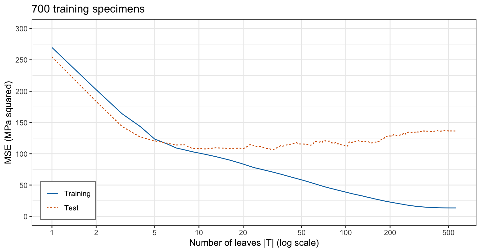
The training MSE falls with every added leaf, to 13.5 for the full tree; it is not zero because specimens with the same age and cement but different other ingredients share a leaf. The test MSE reaches its smallest value, 106.5, at 32 leaves and is higher for larger trees, 136.4 for the full tree. Its smallest leaves hold one or a few specimens each, and their means follow those specimens’ other ingredients and measurement error, not a pattern that recurs in the test specimens.
27.3.2 Cost-complexity pruning
Stopping early is a poor remedy: a split that removes little RSS can lead to splits below it that remove much more, and a stopping rule never sees them. Cost-complexity pruning instead grows \(T_0\) and cuts it back. For each \(\alpha \ge 0\) it finds the subtree \(T \subseteq T_0\) that minimizes
\[C_\alpha(T) = \sum_{\ell=1}^{|T|}\sum_{i:\, x_i \in R_\ell}\left(y_i - \hat y_{R_\ell}\right)^2 + \alpha|T|,\]
where
- \(T\) is a subtree of \(T_0\), obtained by turning some internal nodes into leaves (collapsing everything below them),
- \(|T|\) is the number of leaves of \(T\), and \(R_\ell\) its \(\ell\)th leaf, and
- \(\alpha\) is the tuning parameter, the RSS a leaf must remove to be worth keeping.
With \(\alpha = 0\) the minimizer is \(T_0\), and as \(\alpha\) grows it has fewer leaves, down to the root alone. Like \(\lambda\) in ridge regression and the lasso, \(\alpha\) trades the fit to the training data against a penalty on the model; the penalty counts leaves, as the subset selection criteria count features, rather than measuring the size of estimates. The minimizing subtrees are nested: as \(\alpha\) increases, the next subtree is found by collapsing the internal node whose removal raises the RSS least per leaf removed (weakest link pruning), so the whole sequence comes from one pass over \(T_0\), one subtree per row of the table below.
rpart() scales the tuning parameter by the RSS of the root: its complexity parameter cp is \(\alpha\) divided by the root’s RSS, so a split is kept only if it lowers the RSS by at least cp times the root’s RSS. The default cp = 0.01 is the stopping rule of the default tree, described under Recursive binary splitting.
27.3.3 Cross-validation
While fitting, rpart() also runs 10-fold cross-validation over the sequence of subtrees and stores the results in cptable, which printcp() prints. The full tree’s table has one row per subtree; the rows around the smallest cross-validation estimate are
# The full tree's table, and the rows around its smallest xerror.
cp_table <- full_fit$cptable
best_row <- which.min(cp_table[, "xerror"])
cp_table[best_row + (-2:2), ]
CP nsplit rel error xerror xstd
17 0.005262351 21 0.2978793 0.4307607 0.02853326
18 0.004928922 22 0.2926170 0.4226674 0.02808284
19 0.003547482 23 0.2876881 0.4076152 0.02743197
20 0.003334777 25 0.2805931 0.4134854 0.02712277
21 0.003269014 26 0.2772583 0.4204379 0.02827351
NoteCode
# The cross-validation estimate of the MSE: xerror is the cross-validation
# sum of squared errors divided by the root's RSS.
rss_root <- full_fit$frame$dev[1]
cv_curve <- tibble(leaves = cp_table[, "nsplit"] + 1,
                   cv = cp_table[, "xerror"] * rss_root / n_train)
cv_best <- cv_curve[best_row, ]

# The cross-validation estimate against the number of leaves, the chosen
# size circled, on the axes of the training and test MSE figure.
cv_plot <- ggplot(cv_curve, aes(x = leaves, y = cv)) +
  geom_line() +
  geom_point(data = cv_best, size = 4, shape = 1) +
  leaves_axis +
  mse_axis +
  labs(x = "Number of leaves |T| (log scale)",
       y = "10-fold CV estimate (MPa squared)", title = title_train,
       caption = "Circle: the chosen number of leaves.")
Each row is one subtree of the sequence: CP is the value of cp at which it becomes the minimizer, nsplit its number of splits (one fewer than its number of leaves), rel error its training RSS divided by the root’s RSS, and xerror its cross-validation sum of squared errors divided by the root’s RSS. xstd is a standard error of xerror. The figure plots the cross-validation estimate of the MSE, xerror times the root’s RSS divided by \(n\).
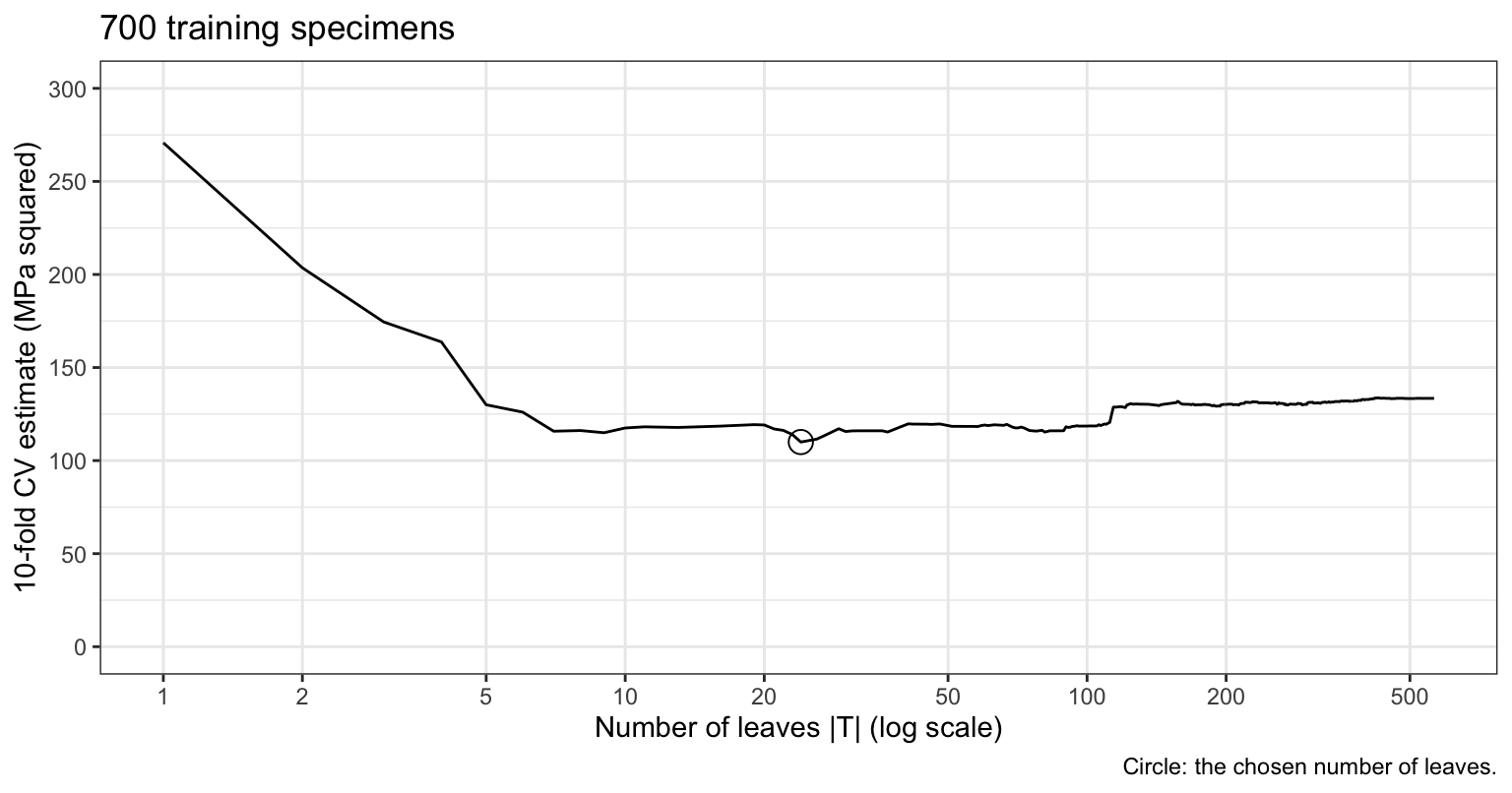
The estimate is smallest, 110.0, at 24 leaves, and it rises for larger trees as the test MSE did. In each fold the full tree is grown from the training folds and pruned with the same values of cp, so the estimate for a value of cp judges the whole procedure, not one particular tree.
27.3.4 Pruned tree
# Prune the full tree at the cp with the smallest xerror.
cp_best <- cp_table[best_row, "CP"]
pruned_fit <- prune(full_fit, cp = cp_best)

# Test MSE of the full and the pruned tree.
y_test <- test$compressive_strength
c(full = mean((y_test - predict(full_fit, test))^2),
  pruned = mean((y_test - predict(pruned_fit, test))^2))
full pruned
136.3742 111.5602
NoteCode
# Least squares on age and cement, for comparison.
two_ls <- lm(compressive_strength ~ age + cement, data = train)

# Test MSE of the trees and of least squares on age and cement.
two_mse <- c(ls = mse(y_test, predict(two_ls, test)),
             default = mse(y_test, predict(two_fit, test)),
             full = mse(y_test, predict(full_fit, test)),
             pruned = mse(y_test, predict(pruned_fit, test)))

# Regions of the pruned tree, with smaller labels, and none on regions
# less than 25 kg per cubic meter tall.
min_height <- 25
pruned_partition <- partition_plot(pruned_fit, label_size = 2.5,
                                   min_height = min_height) +
  labs(caption = paste("Regions less than", min_height,
                       "kg per cubic meter tall are not labeled."))

# The pruned tree's first split, which the prose says is the default
# tree's.
pruned_root <- node_splits(pruned_fit)[1, ]
default_root <- node_splits(two_fit)[1, ]
stopifnot(pruned_root$variable == default_root$variable,
          pruned_root$cut == default_root$cut)

# Share of the full tree's test MSE above the smallest of any subtree that
# pruning removes.
full_excess <- two_mse[["full"]] - test_best$Test
prune_gain <- (two_mse[["full"]] - two_mse[["pruned"]]) / full_excess

# How far the default tree's test MSE is above the smallest of any subtree,
# and a sentence for prose: within near_best counts as near the best size.
near_best <- 0.05
default_excess <- two_mse[["default"]] / test_best$Test - 1
default_text <- if (default_excess <= near_best) {
  paste0("The default tree's test MSE is within ", pct(default_excess, 0),
         " of that smallest value: here the default stopping rules ",
         "happened to stop near the best size.")
} else {
  paste0("The default tree's test MSE is ", pct(default_excess, 0),
         " above that smallest value.")
}
The pruned tree has 24 leaves and test MSE 111.6, against 136.4 for the full tree, 108.5 for the default tree with 9 leaves, and 172.7 for least squares on age and cement, which fits a straight line in age to a curve. The smallest test MSE of any subtree is 106.5. Pruning at the cross-validation choice removes 83% of the full tree’s excess over it. The default tree’s test MSE is within 2% of that smallest value: here the default stopping rules happened to stop near the best size. The figure draws the pruned tree’s regions.
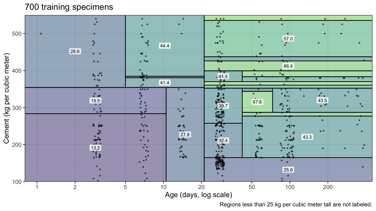
The pruned tree’s first split is the default tree’s, on age at 21 days. Below it, more steps in cement and age divide each side, and some regions are thin bands of cement that hold a few specimens.
NoteBeyond this course
- One-standard-error rule. A common alternative chooses the smallest tree whose
xerroris within onexstdof the smallest, trading a little estimated error for a smaller tree. - The folds.
rpart()draws its folds at random, so the chosen size can change with the seed; itsxvalargument also accepts a vector of fold labels.
27.3.5 All explanatory variables
The same steps on all 8 explanatory variables, the full tree grown and pruned at the smallest cross-validation estimate:
# Grow the full tree on every explanatory variable, then prune at the cp
# with the smallest cross-validation estimate.
all_full <- rpart(compressive_strength ~ ., data = train,
                  control = full_control)
all_cp <- all_full$cptable
all_best <- all_cp[which.min(all_cp[, "xerror"]), "CP"]
all_pruned <- prune(all_full, cp = all_best)
c(test_mse = mean((y_test - predict(all_pruned, test))^2))
test_mse
42.22157 For comparison, least squares on all 8, least squares with \(\log(\texttt{age})\) in place of age, and the default tree:
# Least squares, least squares on log(age), and the default tree.
all_ls <- lm(compressive_strength ~ ., data = train)
log_ls <- lm(compressive_strength ~ . - age + log(age), data = train)
all_default <- rpart(compressive_strength ~ ., data = train)

# Their test MSEs.
fits <- list(ls = all_ls, log_ls = log_ls, default = all_default)
sapply(fits, \(fit) mean((y_test - predict(fit, test))^2))
ls log_ls default
106.36045 48.50664 86.84966
NoteCode
# Test MSE of least squares with log(age).
log_ls_mse <- mse(y_test, predict(log_ls, test))

# Test MSE of each method on both sets of explanatory variables.
all_mse <- c(ls = mse(y_test, predict(all_ls, test)),
             default = mse(y_test, predict(all_default, test)),
             full = mse(y_test, predict(all_full, test)),
             pruned = mse(y_test, predict(all_pruned, test)))
leaves_two <- c(NA, n_leaves(two_fit), n_leaves(full_fit),
                n_leaves(pruned_fit))
leaves_all <- c(NA, n_leaves(all_default), n_leaves(all_full),
                n_leaves(all_pruned))
leaves_text <- function(x) {
  if_else(is.na(x), "none", as.character(x))
}
compare <- tibble(Method = c("Least squares", "Default tree", "Full tree",
                             "Pruned tree"),
                  two_leaves = leaves_text(leaves_two),
                  two_mse = fmt(two_mse, 1),
                  all_leaves = leaves_text(leaves_all),
                  all_mse = fmt(all_mse, 1))
compare_columns <- c("Method",
                     "Leaves, age and cement",
                     "Test MSE, age and cement",
                     paste0("Leaves, all ", p),
                     paste0("Test MSE, all ", p))
compare_table <- knitr::kable(compare, col.names = compare_columns,
                              align = "lrrrr")

# How the pruned tree compares with least squares on log(age), for prose.
log_compare <- if (all_mse[["pruned"]] < log_ls_mse) {
  "does better"
} else {
  "comes close to this error"
}

# Root mean squared error of the pruned tree on all variables, and the
# standard deviation of the test strengths.
all_rmse <- sqrt(all_mse[["pruned"]])
test_sd <- sd(y_test)

# Subtree sizes whose cross-validation estimate is within 5% of the
# smallest.
near_share <- 0.05
all_leaves <- all_cp[, "nsplit"] + 1
all_near <- all_leaves[all_cp[, "xerror"] < (1 + near_share) *
                         min(all_cp[, "xerror"])]

# The prose says the full tree's test MSE is no worse than the pruned
# tree's.
stopifnot(all_mse[["full"]] <= all_mse[["pruned"]])

# Training specimens in each leaf of the full tree: leaves with one
# specimen, and, for the others, whether their specimens share an age,
# share all eight explanatory variables, and share a strength.
leaf_sizes <- table(all_full$where)
n_single <- sum(leaf_sizes == 1)
multi_leaves <- train |>
  mutate(leaf = all_full$where) |>
  filter(leaf %in% as.integer(names(leaf_sizes)[leaf_sizes > 1])) |>
  summarise(same_age = n_distinct(age) == 1,
            same_all = nrow(distinct(pick(all_of(explanatory)))) == 1,
            same_strength = n_distinct(compressive_strength) == 1,
            spread = max(map_dbl(pick(all_of(ingredients)),
                                 \(v) diff(range(v)))),
            .by = leaf)
n_multi <- nrow(multi_leaves)
n_same_all <- sum(multi_leaves$same_all)
n_same_strength <- sum(multi_leaves$same_strength)

# Leaves whose mixes differ by at most close_limit kg per cubic meter in
# every ingredient, how many of those have equal strengths, and the largest
# difference in the others.
close_limit <- 1
is_close <- multi_leaves$spread <= close_limit
n_close <- sum(is_close)
n_close_equal <- sum(is_close & multi_leaves$same_strength)
max_spread <- max(multi_leaves$spread)

# The prose says every leaf with several specimens shares an age.
stopifnot(all(multi_leaves$same_age))
The table collects the test MSE of least squares and of the default, full, and pruned trees, on age and cement and on all 8 explanatory variables.
| Method | Leaves, age and cement | Test MSE, age and cement | Leaves, all 8 | Test MSE, all 8 |
|---|---|---|---|---|
| Least squares | none | 172.7 | none | 106.4 |
| Default tree | 9 | 108.5 | 15 | 86.8 |
| Full tree | 564 | 136.4 | 659 | 40.3 |
| Pruned tree | 24 | 111.6 | 179 | 42.2 |
With all 8 explanatory variables, the pruned tree has 179 leaves and test MSE 42.2, a root mean squared error of 6.5 MPa against a standard deviation of 15.9 MPa among the test strengths. Least squares on the same 8 explanatory variables has test MSE 106.4. The default tree, stopped early by rpart()’s stopping rules at 15 leaves, has test MSE 86.8, against 40.3 and 42.2 for the full and pruned trees grown past it: the splits a stopping rule never reaches are where most of the gain is.
Pruning changes little here. The cross-validation estimate is within 5% of its smallest value for 517 subtrees, with 54 to 659 leaves, so the choice among large trees is loose, and the full tree’s test MSE, 40.3, is no worse than the pruned tree’s. On age and cement alone, specimens that share a small leaf still differ in six ingredients the tree cannot see, and the full tree fits those differences. With all 8 recorded, 619 of the full tree’s 659 leaves hold a single training specimen, and each of the other 40 holds specimens of the same age. In 37 of those 40, the mixes differ by at most 1 kg per cubic meter in every ingredient (5 are identical), and 32 of the 37 have exactly equal strengths; in the other 3, some ingredient differs by up to 99 kg per cubic meter. The full tree therefore predicts a test specimen with the strength of a single training specimen, or the mean of at most 3 specimens of the same age, usually with nearly the same mix. That works here because 68% of the test specimens have a mix that some training specimen also has, often at another age. In this chapter, pruning helped more on age and cement alone, which leave much of the strength unexplained, than on all 8 explanatory variables.
27.4 Classification trees
27.4.1 Penguin species
Question. Which of three species is a penguin, given four measurements of its body?
Data. modeldata::penguins records 344 penguins of three species, Adelie, Chinstrap, and Gentoo, from three islands of the Palmer Archipelago, Antarctica. Each observation is a penguin. The response is species. The explanatory variables are four measurements: bill length and bill depth (mm), flipper length (mm), and body mass (g).
NoteCode
# The four measurements.
measurements <- c("bill_length_mm", "bill_depth_mm", "flipper_length_mm",
                  "body_mass_g")

# Penguins with no measurement at all, and the rest.
penguins_all <- modeldata::penguins
no_measurement <- penguins_all |>
  filter(if_all(all_of(measurements), is.na))
penguins <- penguins_all |>
  filter(!if_all(all_of(measurements), is.na))
n_penguins <- nrow(penguins)

# Penguins kept whose sex is missing, and any other missing measurement.
n_sex_missing <- sum(is.na(penguins$sex))
stopifnot(!anyNA(select(penguins, all_of(measurements))))
2 penguins have none of the four measurements and are removed, leaving 342. Sex is missing for 9 of those; sex is not used, so they stay. Island is not used either, because a split on a categorical variable is not covered in this lecture.
# The training sample size.
n_train_penguins <- 240

# Training penguins: a random sample; every other penguin is a test penguin.
penguin_id <- sample(n_penguins, n_train_penguins)
penguin_train <- penguins[penguin_id, ]
penguin_test <- penguins[-penguin_id, ]
That leaves 240 training penguins and 102 test penguins. The figure plots bill length against flipper length for the training penguins, by species.
NoteCode
# Species colors and shapes.
species_levels <- levels(penguins$species)
species_colors <- setNames(okabe_ito[c(1, 5, 3)], species_levels)
species_shapes <- setNames(c(16, 17, 15), species_levels)

# Flipper length: major lines every 10 mm, minor lines midway.
flipper_limits <- c(170, 235)
flipper_axis <- scale_x_continuous(breaks = seq(170, 230, by = 10),
                                   minor_breaks = seq(175, 235, by = 10),
                                   limits = flipper_limits,
                                   expand = expansion(0))

# Bill length: major lines every 5 mm, minor lines midway.
bill_limits <- c(30, 60)
bill_axis <- scale_y_continuous(breaks = seq(30, 60, by = 5),
                                minor_breaks = seq(32.5, 57.5, by = 5),
                                limits = bill_limits,
                                expand = expansion(0))

# Bill length against flipper length, by species.
title_penguins <- paste(n_train_penguins, "training penguins")
penguin_plot <- ggplot(penguin_train,
                       aes(x = flipper_length_mm, y = bill_length_mm,
                           color = species, shape = species)) +
  geom_point(size = 2) +
  scale_color_manual(values = species_colors) +
  scale_shape_manual(values = species_shapes) +
  flipper_axis +
  bill_axis +
  labs(x = "Flipper length (mm)", y = "Bill length (mm)", color = NULL,
       shape = NULL, title = title_penguins) +
  theme(legend.position = "bottom")

# Training penguins of each species.
species_counts <- table(penguin_train$species)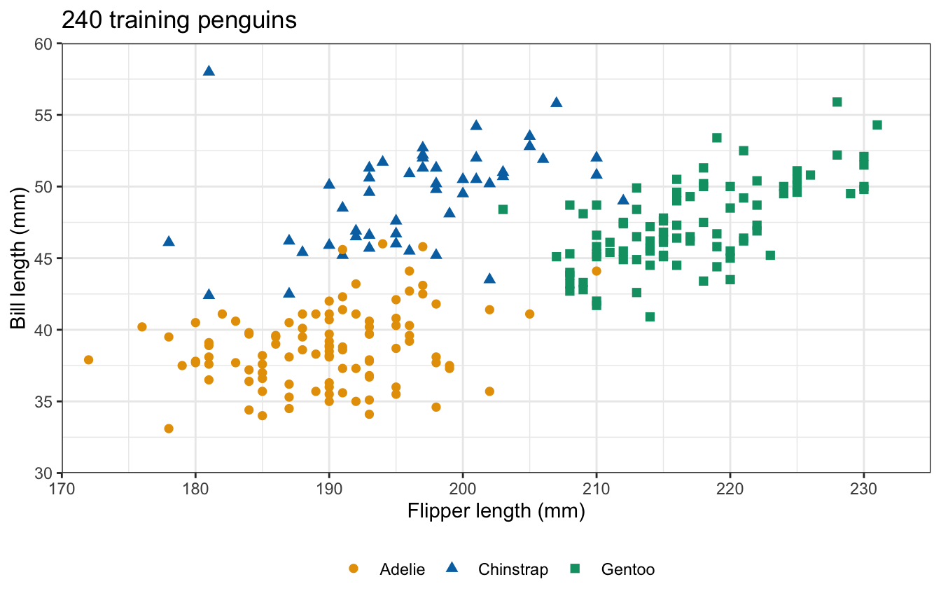
The training penguins are 102 Adelie, 48 Chinstrap, and 90 Gentoo. Gentoo penguins have the longest flippers, and among the shorter-flippered penguins Chinstrap penguins have longer bills than Adelie penguins. One vertical line and one horizontal line in the left part of the plot would separate the three species, with a few penguins on the wrong side.
27.4.2 Most common class
A classification tree splits the explanatory variables into regions in the same way, and predicts for a region its most common class among the training observations in it. The class proportions in a region are
\[\hat p_{\ell k} = \frac{1}{n_\ell}\sum_{i:\, x_i \in R_\ell}\mathrm{I}\left(y_i = k\right),\]
where
- \(K\) is the number of classes, here \(K = 3\), indexed \(k = 1, \ldots, K\),
- \(n_\ell\) is the number of training observations in region \(R_\ell\), and
- \(\hat p_{\ell k}\) is the proportion of them in class \(k\).
The prediction for region \(R_\ell\) is the class \(k\) with the largest \(\hat p_{\ell k}\), and the proportions themselves estimate the probability of each class for an observation in \(R_\ell\).
27.4.3 Node impurity
A regression tree chooses the split with the smallest RSS. A classification tree chooses the split with the smallest impurity, a measure of how mixed the classes in a region are. Three measures of the impurity of region \(\ell\) are
\[E_\ell = 1 - \max_k \hat p_{\ell k}, \qquad G_\ell = \sum_{k=1}^K \hat p_{\ell k}\left(1 - \hat p_{\ell k}\right), \qquad D_\ell = -\sum_{k=1}^K \hat p_{\ell k}\log \hat p_{\ell k},\]
where
- \(E_\ell\) is the classification error rate, the share of the region’s training observations not in its most common class,
- \(G_\ell\) is the Gini index, and
- \(D_\ell\) is the entropy, with the natural log and \(0\log 0 = 0\).
All three are zero when every observation in the region is in one class (a pure node), and largest when the classes are equally common. The impurity of a split is the average of the impurities of its two regions, weighted by their numbers of observations, \(\left(n_1 Q_1 + n_2 Q_2\right)/\left(n_1 + n_2\right)\), where \(Q\) is any of the three measures and \(Q_1\) and \(Q_2\) are its values in the two regions.
NoteCode
# The three impurity measures of a vector of class proportions.
error_rate <- function(prop) {
  1 - max(prop)
}
gini <- function(prop) {
  sum(prop * (1 - prop))
}
entropy <- function(prop) {
  positive <- prop[prop > 0]
  -sum(positive * log(positive))
}

# Class counts and the three impurities of a set of penguins.
node_row <- function(node, species) {
  counts <- table(species)
  prop <- counts / sum(counts)
  tibble(Node = node, Adelie = counts[["Adelie"]],
         Chinstrap = counts[["Chinstrap"]], Gentoo = counts[["Gentoo"]],
         n = sum(counts), error = error_rate(prop), gini = gini(prop),
         entropy = entropy(prop))
}

# Impurity removed by every cut point of measurement v, for the penguins in
# `data`, by one impurity measure: the impurity before the split minus the
# weighted impurity after it, as a share of the impurity before.
class_split_curve <- function(data, v, measure) {
  values <- sort(unique(data[[v]]))
  cuts <- (head(values, -1) + tail(values, -1)) / 2
  impurity <- function(species) {
    measure(table(species) / length(species))
  }
  before <- impurity(data$species)
  after <- map_dbl(cuts, \(s) {
    left <- data[[v]] < s
    (sum(left) * impurity(data$species[left]) +
       sum(!left) * impurity(data$species[!left])) / nrow(data)
  })
  # Rounding sets rounding error in an unchanged impurity to exactly 0.
  share <- round((before - after) / before, 12)
  tibble(variable = v, cut = cuts, share = share)
}

# The best Gini split of the training penguins over all four measurements.
root_gini <- map(measurements, \(v) {
  class_split_curve(penguin_train, v, gini)
}) |>
  list_rbind() |>
  slice_max(share, n = 1, with_ties = FALSE)
root_var <- root_gini$variable
root_cut <- root_gini$cut

# The root, its two children, and the weighted average of the children.
goes_left <- penguin_train[[root_var]] < root_cut
left_label <- paste("flipper <", root_cut)
right_label <- paste("flipper >=", root_cut)
node_rows <- bind_rows(node_row("Root", penguin_train$species),
                       node_row(left_label, penguin_train$species[goes_left]),
                       node_row(right_label,
                                penguin_train$species[!goes_left]))
weights <- node_rows$n[2:3] / node_rows$n[1]
split_row <- node_rows[2:3, ] |>
  summarise(across(c(error, gini, entropy), \(x) sum(weights * x))) |>
  mutate(Node = "Split (weighted)")
impurity_tibble <- bind_rows(node_rows, split_row) |>
  mutate(across(c(error, gini, entropy), \(x) fmt(x, 3)),
         across(c(Adelie, Chinstrap, Gentoo, n), \(x) {
           if_else(is.na(x), "", as.character(x))
         }))
impurity_table <- knitr::kable(impurity_tibble,
                               col.names = c("Node", "Adelie", "Chinstrap",
                                             "Gentoo", "n", "Error rate",
                                             "Gini index", "Entropy"),
                               align = "lrrrrrrr")

# Share of each impurity removed by the split.
share_removed <- function(measure) {
  1 - split_row[[measure]] / node_rows[[measure]][1]
}
The best split of the training penguins by the Gini index is on flipper_length_mm at 206.5 mm. The table gives the class counts and the three impurities of the root, of its two children, and of the split.
| Node | Adelie | Chinstrap | Gentoo | n | Error rate | Gini index | Entropy |
|---|---|---|---|---|---|---|---|
| Root | 102 | 48 | 90 | 240 | 0.575 | 0.639 | 1.053 |
| flipper < 206.5 | 101 | 44 | 1 | 146 | 0.308 | 0.431 | 0.651 |
| flipper >= 206.5 | 1 | 4 | 89 | 94 | 0.053 | 0.102 | 0.234 |
| Split (weighted) | 0.208 | 0.302 | 0.488 |
The right child is nearly pure Gentoo, and the left child holds nearly all the Adelie and Chinstrap penguins. The split removes 64% of the root’s error rate, 53% of its Gini index, and 54% of its entropy.
27.4.4 Gini index and entropy
The figure plots, for every cut point on bill length within the left child, the share of the left child’s impurity that a split there removes, by each measure.
NoteCode
# The penguins of the left child, and the three curves on bill length.
left_child <- penguin_train[goes_left, ]
measure_names <- c("Error rate", "Gini index", "Entropy")
measures <- list(error_rate, gini, entropy)
impurity_curves <- map2(measures, measure_names, \(measure, name) {
  class_split_curve(left_child, "bill_length_mm", measure) |>
    mutate(measure = name)
}) |>
  list_rbind() |>
  mutate(measure = factor(measure, levels = measure_names))

# Cut points at which the error rate removes nothing but the Gini index
# removes some impurity.
error_flat <- impurity_curves |>
  pivot_wider(names_from = measure, values_from = share) |>
  filter(`Error rate` <= 0, `Gini index` > 0)

# The prose says the error rate removes nothing at every cut point up to
# the largest of these.
low_error <- impurity_curves |>
  filter(measure == "Error rate", cut <= max(error_flat$cut))
stopifnot(all(low_error$share <= 0))

# Bill length: the left child's range, major lines every 5 mm, minor lines
# midway.
bill_x_axis <- scale_x_continuous(breaks = seq(30, 60, by = 5),
                                  minor_breaks = seq(32.5, 57.5, by = 5))

# Share removed: major lines every 20%, minor lines midway.
removed_axis <- scale_y_continuous(breaks = seq(0, 1, by = 0.2),
                                   minor_breaks = seq(0.1, 0.9, by = 0.2),
                                   limits = c(0, 1),
                                   labels = scales::label_percent())
title_left <- paste(nrow(left_child), "training penguins with",
                    left_label, "mm")
impurity_plot <- ggplot(impurity_curves,
                        aes(x = cut, y = share, color = measure,
                            linetype = measure)) +
  geom_line(linewidth = 0.8) +
  scale_color_manual(values = okabe_ito[c(4, 5, 3)]) +
  bill_x_axis +
  removed_axis +
  labs(x = "Cut point s on bill length (mm)",
       y = "Share of impurity removed", color = NULL, linetype = NULL,
       title = title_left) +
  theme(legend.position = "bottom")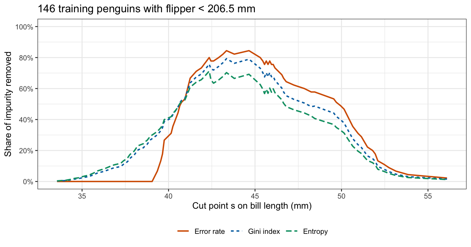
All three measures are largest near the same cut point, which separates Adelie from Chinstrap. Away from it they differ. At every cut point up to 39.05 mm the error rate removes nothing: both regions keep Adelie as their most common class, so the count of penguins outside it does not change. The Gini index and the entropy still fall at those cut points, because one region becomes purer.
The reason is concavity. The class proportions of a region are the weighted average of those of its two parts, \(\hat p_k = \left(n_1\hat p_{1k} + n_2\hat p_{2k}\right)/\left(n_1 + n_2\right)\), with \(\hat p_{1k}\) and \(\hat p_{2k}\) the proportions of class \(k\) in the two parts. The Gini index and the entropy are strictly concave functions of the proportions, so by Jensen’s inequality the weighted impurity after a split is smaller than before unless the two parts have the same proportions. The error rate is concave but linear wherever the most common class stays the same, so a split that leaves both parts with the parent’s most common class does not lower it. A tree grown on the error rate can stop at a split like that, while splits below it would separate the classes. rpart() grows a classification tree with the Gini index by default; parms = list(split = "information") uses the entropy. The error rate is the usual measure for pruning, where the goal is prediction accuracy.
27.4.5 Fitting
# A classification tree on the four measurements.
penguin_fit <- rpart(species ~ bill_length_mm + bill_depth_mm +
                       flipper_length_mm + body_mass_g,
                     data = penguin_train, method = "class")
print(penguin_fit, digits = 4)
n= 240
node), split, n, loss, yval, (yprob)
* denotes terminal node
1) root 240 138 Adelie (0.425000 0.200000 0.375000)
2) flipper_length_mm< 206.5 146 45 Adelie (0.691781 0.301370 0.006849)
4) bill_length_mm< 43.35 99 2 Adelie (0.979798 0.020202 0.000000) *
5) bill_length_mm>=43.35 47 5 Chinstrap (0.085106 0.893617 0.021277) *
3) flipper_length_mm>=206.5 94 5 Gentoo (0.010638 0.042553 0.946809)
6) bill_depth_mm>=17.05 7 3 Chinstrap (0.142857 0.571429 0.285714) *
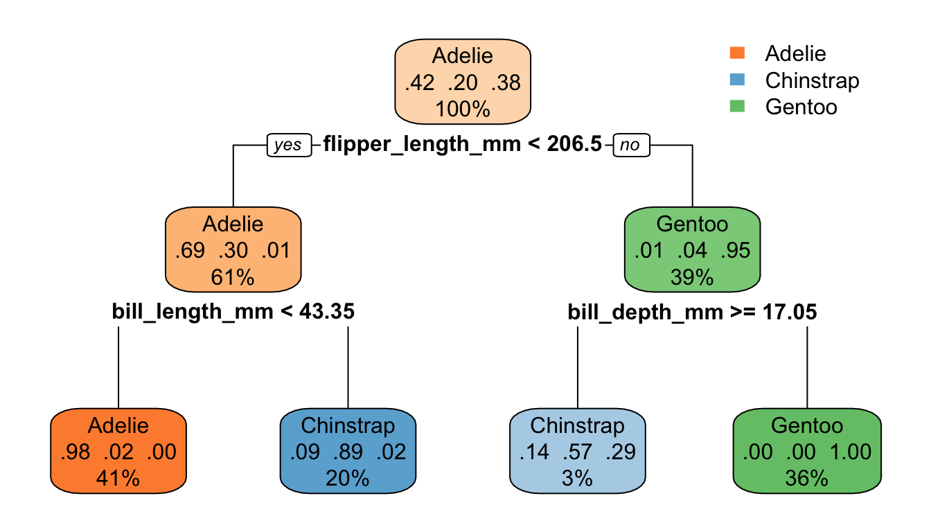
7) bill_depth_mm< 17.05 87 0 Gentoo (0.000000 0.000000 1.000000) *Each line gives a node’s number of training penguins, the number not in its most common class (loss), that class (yval), and the class proportions \(\hat p_{\ell k}\) in the order Adelie, Chinstrap, and Gentoo. The tree has 4 leaves and splits on flipper_length_mm, bill_length_mm, and bill_depth_mm; body_mass_g is not used. Its first split is the one in the impurity table. The diagram shows the most common class of each node, its class proportions, and its share of the training penguins.
NoteCode
# Regions of the penguin tree, shaded by their predicted species, over the
# training penguins.
penguin_limits <- list(flipper_length_mm = flipper_limits,
                       bill_length_mm = bill_limits)
species_of <- attr(penguin_fit, "ylevels")

# Node 3 is split on bill depth, which the plot does not show; it is drawn
# as one region.
penguin_plane <- snip.rpart(penguin_fit, toss = 3)
plane_vars <- setdiff(unique(as.character(penguin_plane$frame$var)),
                      "<leaf>")
stopifnot(all(plane_vars %in% names(penguin_limits)))
penguin_rectangles <- leaf_rectangles(penguin_plane, penguin_limits) |>
  mutate(species = factor(species_of[value], levels = species_levels))
penguin_partition <- ggplot() +
  geom_rect(data = penguin_rectangles,
            aes(xmin = xmin, xmax = xmax, ymin = ymin, ymax = ymax,
                fill = species),
            alpha = 0.15, color = "black", show.legend = FALSE) +
  geom_point(data = penguin_train,
             aes(x = flipper_length_mm, y = bill_length_mm,
                 color = species, shape = species),
             size = 2) +
  scale_fill_manual(values = species_colors) +
  scale_color_manual(values = species_colors) +
  scale_shape_manual(values = species_shapes) +
  flipper_axis +
  bill_axis +
  labs(x = "Flipper length (mm)", y = "Bill length (mm)", color = NULL,
       shape = NULL, title = title_penguins) +
  theme(legend.position = "bottom")
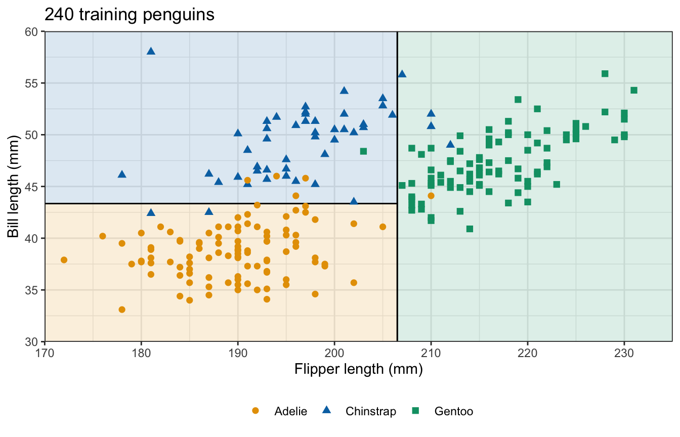
The figure draws the tree’s regions over the data plot, each shaded by its predicted species. The region of long flippers is drawn as one rectangle: its split on bill depth, a measurement the plot does not show, is left out.
27.4.6 Test confusion matrix
# Predicted species of the test penguins, against their species.
penguin_pred <- predict(penguin_fit, penguin_test, type = "class")
confusion <- table(Predicted = penguin_pred,
                   Observed = penguin_test$species)
confusion
Observed
Predicted Adelie Chinstrap Gentoo
Adelie 48 3 0
Chinstrap 1 17 1
Gentoo 0 0 32mean(penguin_pred == penguin_test$species)[1] 0.9509804
NoteCode
# Accuracy, misclassified test penguins, and the most common test species.
accuracy <- mean(penguin_pred == penguin_test$species)
n_wrong <- sum(penguin_pred != penguin_test$species)
majority_share <- max(table(penguin_test$species)) / nrow(penguin_test)
The tree classifies 95.1% of the 102 test penguins correctly and misclassifies 5. Predicting the most common species for every penguin would be right for 48.0% of them.
27.4.7 Pruning
A classification tree is pruned in the same way, with the error rate in place of the RSS in \(C_\alpha(T)\). The rows of the full tree’s table from two above its smallest cross-validation estimate to the full tree are
# The full classification tree, and its table from two rows above the
# smallest xerror.
penguin_full <- rpart(species ~ bill_length_mm + bill_depth_mm +
                        flipper_length_mm + body_mass_g,
                      data = penguin_train, method = "class",
                      control = full_control)
penguin_cp <- penguin_full$cptable
penguin_best <- which.min(penguin_cp[, "xerror"])
penguin_cp[max(1, penguin_best - 2):nrow(penguin_cp), ]
CP nsplit rel error xerror xstd
2 0.275362319 1 0.362318841 0.36231884 0.04559079
3 0.028985507 2 0.086956522 0.12318841 0.02879998
4 0.010869565 3 0.057971014 0.07246377 0.02243258
5 0.007246377 5 0.036231884 0.07246377 0.02243258
6 0.003623188 9 0.007246377 0.07971014 0.02347629
7 0.000000000 11 0.000000000 0.07246377 0.02243258
NoteCode
# The subtree with the smallest cross-validation estimate, and its test
# accuracy.
penguin_pruned <- prune(penguin_full, cp = penguin_cp[penguin_best, "CP"])
test_accuracy <- function(fit) {
  predicted <- predict(fit, penguin_test, type = "class")
  mean(predicted == penguin_test$species)
}
pruned_accuracy <- test_accuracy(penguin_pruned)

# Training penguins misclassified at the root, and in cross-validation by
# each subtree; the row of the subtree with the default tree's size.
train_counts <- table(penguin_train$species)
root_class <- names(which.max(train_counts))
root_errors <- n_train_penguins - max(train_counts)
cv_errors <- round(penguin_cp[, "xerror"] * root_errors)

# Every size that ties for the smallest estimate; which.min() takes the
# first, the smallest tree.
penguin_leaves <- penguin_cp[, "nsplit"] + 1
tied_leaves <- penguin_leaves[cv_errors == min(cv_errors)]
tie_text <- if (length(tied_leaves) > 1) {
  paste0(" (", and_list(tied_leaves), " leaves tie, and the smallest tree ",
         "is taken)")
} else {
  ""
}

# Whether the smallest estimate is at the full tree.
best_is_full <- penguin_best == nrow(penguin_cp)
if (best_is_full) {
  tie_text <- paste0(tie_text, ", the full tree itself, so here pruning ",
                     "removes nothing")
}

# Node 3's split in the default and the chosen tree, as code for prose,
# and the number of training penguins in node 6, its first child.
node_3_text <- function(fit) {
  split <- filter(node_splits(fit), node == 3)
  label <- labels(fit)[rownames(fit$frame) == "6"]
  op <- if (str_detect(label, ">=")) ">=" else "<"
  paste(split$variable, op, cut_text(split$cut))
}
node_6_size <- function(fit) {
  fit$frame$n[rownames(fit$frame) == "6"]
}
default_3 <- node_3_text(penguin_fit)
pruned_3 <- node_3_text(penguin_pruned)

# Test penguins each tree classifies correctly.
n_right <- function(fit) {
  predicted <- predict(fit, penguin_test, type = "class")
  sum(predicted == penguin_test$species)
}

# The prose compares two trees of the same size that differ only in node
# 3, whose chosen-tree child is smaller than the default minbucket allows.
minbucket <- rpart.control()$minbucket
stopifnot(n_leaves(penguin_pruned) == n_leaves(penguin_fit),
          default_3 != pruned_3,
          node_6_size(penguin_pruned) < minbucket)
For a classification tree, rel error and xerror are numbers of misclassified training penguins divided by the root’s, the 138 penguins that are not Adelie. The smallest cross-validation estimate, 10 misclassified training penguins, is at 4 leaves (4, 6, and 12 leaves tie, and the smallest tree is taken); the default tree has 4. The two trees differ in node 3: the default tree splits it at bill_depth_mm >= 17.05, leaving a leaf of 7 penguins, and the chosen tree at bill_depth_mm >= 17.65, leaving a leaf of 5, which the default minbucket = 7 forbids. The chosen tree classifies 96.1% of the test penguins correctly, against 95.1% for the default tree, 98 of 102 against 97.
27.5 Strengths and weaknesses
27.5.1 Interpretability
A small tree is a list of rules a reader can follow without software: the default concrete tree on age and cement has 9 leaves, and the default penguin tree 4. A classification tree handles any number of classes with no change to the method. Interpretability fades with size: the pruned tree on all 8 explanatory variables has 179 leaves, more than anyone reads.
27.5.2 Nonlinearity and interactions
A tree needs no features built for curvature or interaction. On all 8 explanatory variables the pruned tree’s test MSE was 42.2, against 106.4 for least squares. Least squares with \(\log(\texttt{age})\) in place of age, a feature chosen after seeing the curve in the data plot, has test MSE 48.5; the tree does better without being told about the curvature.
NoteCode
# Whether node n is node a or lies below it.
is_below <- function(n, a) {
  depth_gap <- floor(log2(n)) - floor(log2(a))
  depth_gap >= 0 & floor(n / 2^depth_gap) == a
}

# Cement cut points below the young (node 2) and the old (node 3) branch.
two_splits <- node_splits(two_fit)
stopifnot(two_splits$variable[1] == "age",
          abs(two_splits$cut[1] - best_age$cut) < 1e-8)
cement_splits <- filter(two_splits, variable == "cement")
young_cuts <- sort(cement_splits$cut[is_below(cement_splits$node, 2)])
old_cuts <- sort(cement_splits$cut[is_below(cement_splits$node, 3)])
A split on another variable below a split is an interaction. In the default tree on age and cement, the specimens younger than 21 days are split on cement at 354.5 kg per cubic meter, and the older ones at 164.8, 257.7, and 352.5: the step in strength that cement makes depends on age.
27.5.3 Step functions
NoteCode
# Number of random halvings of the training specimens.
n_halvings <- 200

# For each halving, the default trees and least squares on age and cement
# fit to the two halves; their first splits, and the root mean squared
# difference of the two fits' predictions for the test specimens.
two_formula <- compressive_strength ~ age + cement
rms_gap <- function(a, b) {
  sqrt(mean((predict(a, test) - predict(b, test))^2))
}
halvings <- map(seq_len(n_halvings), \(b) {
  half <- sample(n_train, n_train / 2)
  tree_a <- rpart(two_formula, data = train[half, ])
  tree_b <- rpart(two_formula, data = train[-half, ])
  ls_a <- lm(two_formula, data = train[half, ])
  ls_b <- lm(two_formula, data = train[-half, ])
  tibble(halving = b,
         root_a = labels(tree_a)[2],
         root_b = labels(tree_b)[2],
         tree_gap = rms_gap(tree_a, tree_b),
         ls_gap = rms_gap(ls_a, ls_b),
         trees = list(list(tree_a, tree_b)),
         halves = list(half))
}) |>
  list_rbind()

# How often the first splits of the two halves agree, and the most common
# first split.
root_labels <- c(halvings$root_a, halvings$root_b)
root_counts <- sort(table(root_labels), decreasing = TRUE)
same_root <- mean(halvings$root_a == halvings$root_b)
mean_tree_gap <- mean(halvings$tree_gap)
mean_ls_gap <- mean(halvings$ls_gap)

# Predicted strength at 28 days for cement on a grid.
cement_grid <- tibble(age = 28, cement = seq(100, 550, by = 0.5))

# The first 20 halvings: predictions of their 40 trees at 28 days.
n_shown <- 20
shown_curves <- map(seq_len(n_shown), \(b) {
  map(1:2, \(h) {
    tree <- halvings$trees[[b]][[h]]
    mutate(cement_grid, strength = predict(tree, cement_grid),
           curve = paste(b, h))
  }) |>
    list_rbind()
}) |>
  list_rbind()

# The default tree and least squares on all training specimens.
fit_curves <- bind_rows(
  mutate(cement_grid, strength = predict(two_fit, cement_grid),
         fit = "Default tree"),
  mutate(cement_grid, strength = predict(two_ls, cement_grid),
         fit = "Least squares")
) |>
  mutate(fit = factor(fit, levels = c("Default tree", "Least squares")))

# Training specimens tested at 28 days.
train_28 <- filter(train, age == 28)
title_28 <- paste(nrow(train_28), "training specimens tested at 28 days")

# Predicted strength against cement at 28 days, over those specimens.
step_base <- ggplot(train_28, aes(x = cement, y = compressive_strength)) +
  geom_point(alpha = 0.3, size = 1) +
  cement_axis +
  strength_axis +
  labs(x = "Cement (kg per cubic meter)",
       y = "Strength at 28 days (MPa)", title = title_28)
step_fits <- step_base +
  geom_line(data = fit_curves,
            aes(y = strength, color = fit, linetype = fit),
            linewidth = 0.9) +
  scale_color_manual(values = okabe_ito[c(5, 4)]) +
  labs(color = NULL, linetype = NULL) +
  theme(legend.position = "inside",
        legend.position.inside = c(0.99, 0.03),
        legend.justification = c(1, 0),
        legend.background = element_rect(color = "grey50"))
step_halves <- step_base +
  geom_line(data = shown_curves, aes(y = strength, group = curve),
            color = okabe_ito[5], alpha = 0.4)
step_aligned <- patchwork::align_patches(step_fits, step_halves)
A halving splits the 700 training specimens at random into two halves of 350. The tabs plot predicted strength at 28 days against cement, over the training specimens tested at that age. The first tab draws the default tree and least squares on age and cement, fit to all 700 training specimens; the second draws the default trees fit to the 40 halves of 20 halvings.
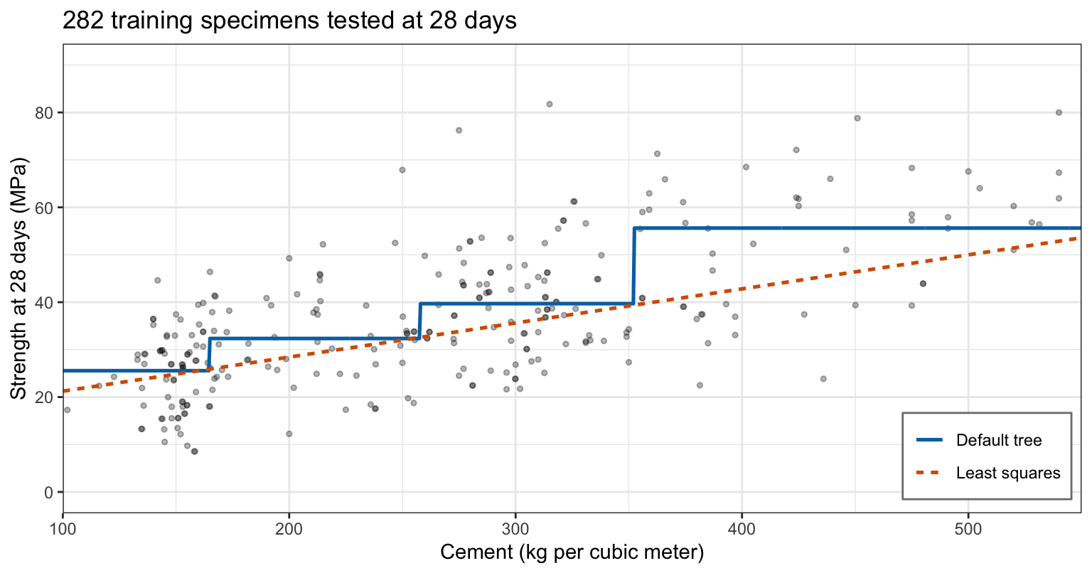
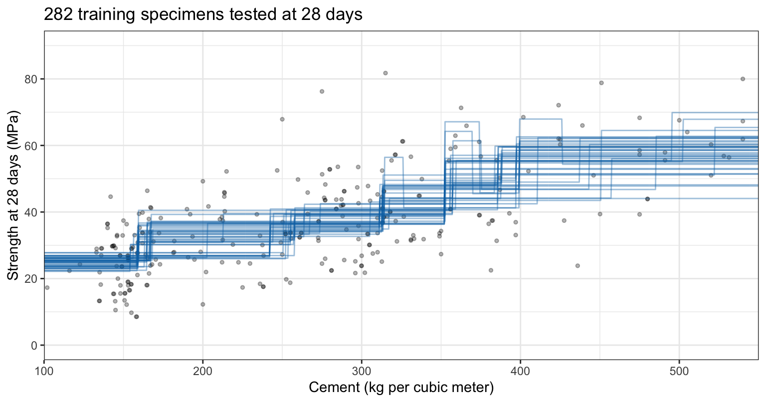
The tree’s prediction is flat between cut points and jumps at each one, so two mixes on either side of a cut point get different predictions however close they are, and two mixes far apart within a region get the same one. Least squares draws a straight line through the same specimens.
27.5.4 Instability
The trees on halves in the second tab above differ in where they put their steps and how high each step is. The tabs draw the regions of the two trees of one halving, each over its own half of the training specimens: the first halving, in the order drawn, whose two trees split first in different places.
NoteCode
# The first halving whose two trees split first in different places.
shown <- which(halvings$root_a != halvings$root_b)[1]

# Its two halves, and the regions of their trees.
first_half <- halvings$halves[[shown]]
title_half <- paste(n_train / 2, "training specimens")
half_plots <- map(1:2, \(h) {
  rows <- if (h == 1) first_half else -first_half
  partition_plot(halvings$trees[[shown]][[h]], data = train_plot[rows, ],
                 title = title_half)
})

# The first split and the number of leaves of each tree.
half_roots <- c(halvings$root_a[shown], halvings$root_b[shown])
half_leaves <- map_int(halvings$trees[[shown]], n_leaves)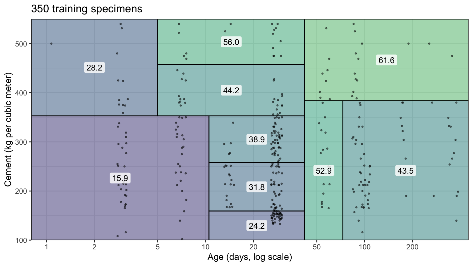
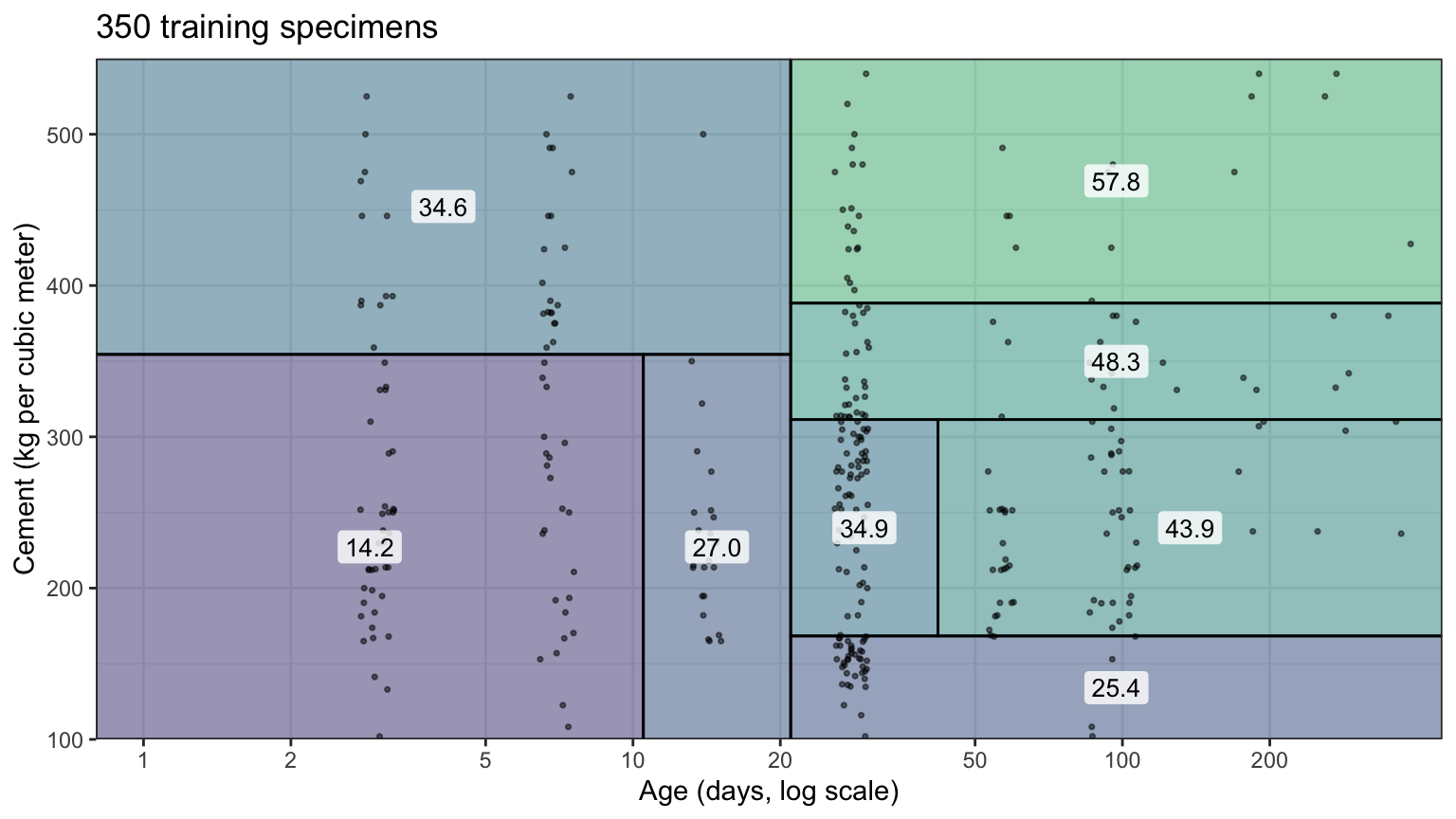
The tree on the first half splits first on age< 42 and has 10 leaves; the tree on the second half splits first on age< 21 and has 8. Each later split is made inside a region the first split creates, so the two partitions differ throughout. Over 200 random halvings, the two halves split first at the same place 50% of the time; the most common first split, age< 21, is the first split of 74% of the 400 trees. Their predictions for a test specimen differ by 6.2 MPa on average (root mean square over the test specimens, averaged over the halvings). Least squares fits to the same halves differ by 1.6 MPa.
A tree has high variance: trees fit to different training samples, shown here by the two halves of a halving, differ, because each split is chosen from the data and a different first or second split changes every split below it. The next lecture averages many trees to reduce that variance.
NoteBeyond this course
- Missing values.
rpart()keeps an observation with a missing value of the split’s explanatory variable by sending it down a surrogate split, a split on another explanatory variable that best mimics the primary one;print(summary(fit))lists them. - Categorical explanatory variables. A split on a categorical variable sends a subset of its levels left and the rest right; for a numeric response the levels can be ordered by their mean response, which reduces the search to splits of that order.
- Conditional inference trees. The
partykitpackage chooses each split by a hypothesis test of association between the response and each explanatory variable, which avoids favoring variables with many possible cut points. - Other trees. Trees with splits on linear combinations of the explanatory variables, and trees with a linear model in each leaf, trade some interpretability for smoother fits.
27.6 Conclusion
A decision tree divides the values of the explanatory variables into rectangular regions and predicts a constant in each: the mean training response of the region for a regression tree, and its most common class for a classification tree, whose class proportions estimate the class probabilities. It splits on the explanatory variables as recorded, so it needs no features built by hand.
The regions are grown by recursive binary splitting, a greedy, top-down search. Each split chooses one explanatory variable and one cut point to minimize the RSS of the two new regions, which is the same as maximizing \(n_1n_2\left(\bar y_1 - \bar y_2\right)^2/\left(n_1 + n_2\right)\), or, for classes, to minimize the weighted Gini index or entropy. Those two measures, unlike the classification error rate, are strictly concave in the class proportions, so they reward any split that makes a region purer.
A tree grown until its leaves are tiny can fit the training data too closely; how much this costs depends on how much variation the explanatory variables leave for small leaves to fit. Cost-complexity pruning cuts it back by minimizing the training RSS (or error) plus \(\alpha\) times the number of leaves, which gives a nested sequence of subtrees from the full tree at \(\alpha = 0\) to the root. The tuning parameter, cp in rpart(), is chosen by 10-fold cross-validation and the chosen tree evaluated once on test data.
Trees are easy to read when they are small, capture nonlinearity and interactions without feature engineering, and handle any number of classes. Their predictions are step functions, and they have high variance: a different training sample can change the first splits and, through them, every region below.
The next lecture reduces that variance by averaging many trees: bagging fits a tree to each of many bootstrap samples, and random forests also restrict each split to a random subset of the explanatory variables.