24 Principal Components Regression and Partial Least Squares

Learning objectives

After this lecture you should be able to

define principal components regression, write its model $y_i = \theta_0 + \sum_{m=1}^M\theta_m z_{im} + \epsilon_i$ on the first $M$ principal component scores, and derive each estimate $\hat\theta_m$ as the simple regression estimate on the $m$th scores, with variance $\sigma^2/(nv_m)$,
show that principal components regression is a linear model in the standardized features with estimate $\boldsymbol{\Phi}_M\hat\theta$, and explain why $M = p$ gives least squares, why it is not variable selection, and when dropping a component lowers the mean squared error of the fitted values about the true mean at the training observations,
choose $M$ by $k$-fold cross-validation with the standardization and the directions recomputed from the training folds in each fold, and explain why computing partial least squares directions from all the training data makes the cross-validation estimate optimistic,
derive the first partial least squares direction as the unit vector whose scores have the largest squared sample covariance with the response, compute it from the simple regression estimates, and contrast it with the first principal component and with the least squares direction,
describe how the later partial least squares directions are found from the residuals of the features, and describe why directions chosen with the response can lower the bias of a fit with $M$ directions but can add variance, and
derive the factor $v_m/(v_m + \lambda/n)$ by which ridge regression shrinks the fit along each principal component, and compare principal components regression, partial least squares, and ridge regression by which directions each favors and how it treats them.

The Principal Components lecture replaced the $p$ standardized features $\tilde x_{ij}$ by their principal components. The loading vectors $\phi_1, \ldots, \phi_p$ are the eigenvectors of the sample correlation matrix $\mathbf{R}$, ordered by the variances $v_1 \ge \cdots \ge v_p$ of their scores $z_{im} = \tilde x_i\phi_m$; the scores of different components are uncorrelated, and the variances sum to $p$. Price played no part in finding them, and the lecture ended with a finding about price: a late component with little variance, PC4, was more strongly correlated with price than PC2 or PC3, and, because the scores are uncorrelated, the squared correlations of price with the six scores summed to the $R^2$ of the least squares regression of price on all six scores.

This lecture regresses a response on the first $M$ components, principal components regression (PCR), and then on $M$ directions chosen with the response, partial least squares (PLS). Both are dimension reduction methods: they fit least squares to $M < p$ linear combinations of the features instead of to the features themselves. As in the principal components lecture, $M$ is the number of components or directions kept; in the ridge and lasso lectures it was the number of repeated training samples.

24.1 Diamond prices

24.1.1 Data

Question. From a small training sample, how well do a diamond’s six numeric measurements predict its price, and does regressing on a few linear combinations of them predict better than regressing on all six?

Data. The diamonds are those of the principal components lecture: ggplot2::diamonds, with the diamonds that have a dimension of 0 or larger than 20 mm removed. The explanatory variables are again weight (carat), total depth percentage (depth), table percentage (table), and the length, width, and depth in mm (x, y, and z; the depth z is a distance, the column depth a percentage). In code font these are the recorded columns, while $y_i$ and $z_{im}$ in math are the response and the scores. The response is the price, price, in US dollars.

Code

# The numeric explanatory variables, and the largest plausible dimension.
features <- c("carat", "depth", "table", "x", "y", "z")
p <- length(features)
max_mm <- 20

# Remove diamonds with a dimension of 0 or above max_mm, as in the
# principal components lecture, and add the log price.
kept <- diamonds |>
  filter(x > 0, y > 0, z > 0) |>
  filter(x <= max_mm, y <= max_mm, z <= max_mm) |>
  mutate(log_price = log(price))
n_kept <- nrow(kept)
n_removed <- nrow(diamonds) - n_kept

That removes 23 of the 53,940 diamonds and leaves 53,917. The test diamonds are split off before any plotting or fitting.

# The training sample size.
n_train <- 100

# Training diamonds: a random sample; every other diamond is a test diamond.
train_id <- sample(n_kept, n_train)
train <- kept[train_id, ]
test <- kept[-train_id, ]
n_test <- nrow(test)

# Folds for 10-fold cross-validation of the training diamonds.
n_folds <- 10
fold_labels <- rep(seq_len(n_folds), length.out = n_train)
fold_id <- sample(fold_labels)

These sample() calls are the first random draws after set.seed(20261022). That leaves 100 training diamonds and 53,817 test diamonds. The training sample size is that of the ridge and lasso lectures; the least squares section below says why it is small. The tabs plot the price and the log price of the training diamonds against each explanatory variable.

Code

# Panel labels: each explanatory variable and its unit.
units <- c(carat = "carats",
           depth = "%",
           table = "%",
           x = "mm",
           y = "mm",
           z = "mm")
panel_labels <- paste0(features, " (", units, ")")

# One row per training diamond and explanatory variable.
train_long <- train |>
  pivot_longer(all_of(features), names_to = "variable") |>
  mutate(variable = factor(variable, levels = features, labels = panel_labels))

# A response against each explanatory variable, one panel each.
title_train <- paste(n_train, "training diamonds")
response_plot <- function(response, label) {
  ggplot(train_long, aes(x = value, y = .data[[response]])) +
    geom_point(alpha = 0.6, size = 1) +
    facet_wrap(~ variable, scales = "free_x", nrow = 2) +
    labs(x = NULL,
         y = label,
         title = title_train) +
    theme(panel.spacing.x = unit(1.5, "lines"))
}
price_plot <- response_plot("price", "Price (US dollars)") +
  scale_y_continuous(labels = scales::label_dollar())
log_price_plot <- response_plot("log_price", "Log price, log(US dollars)")

# Mean, median, and largest training price, and the price of the heaviest
# training diamond.
price_summary <- c(mean = mean(train$price),
                   median = median(train$price),
                   max = max(train$price))
heaviest <- which.max(train$carat)
heaviest_price <- train$price[heaviest]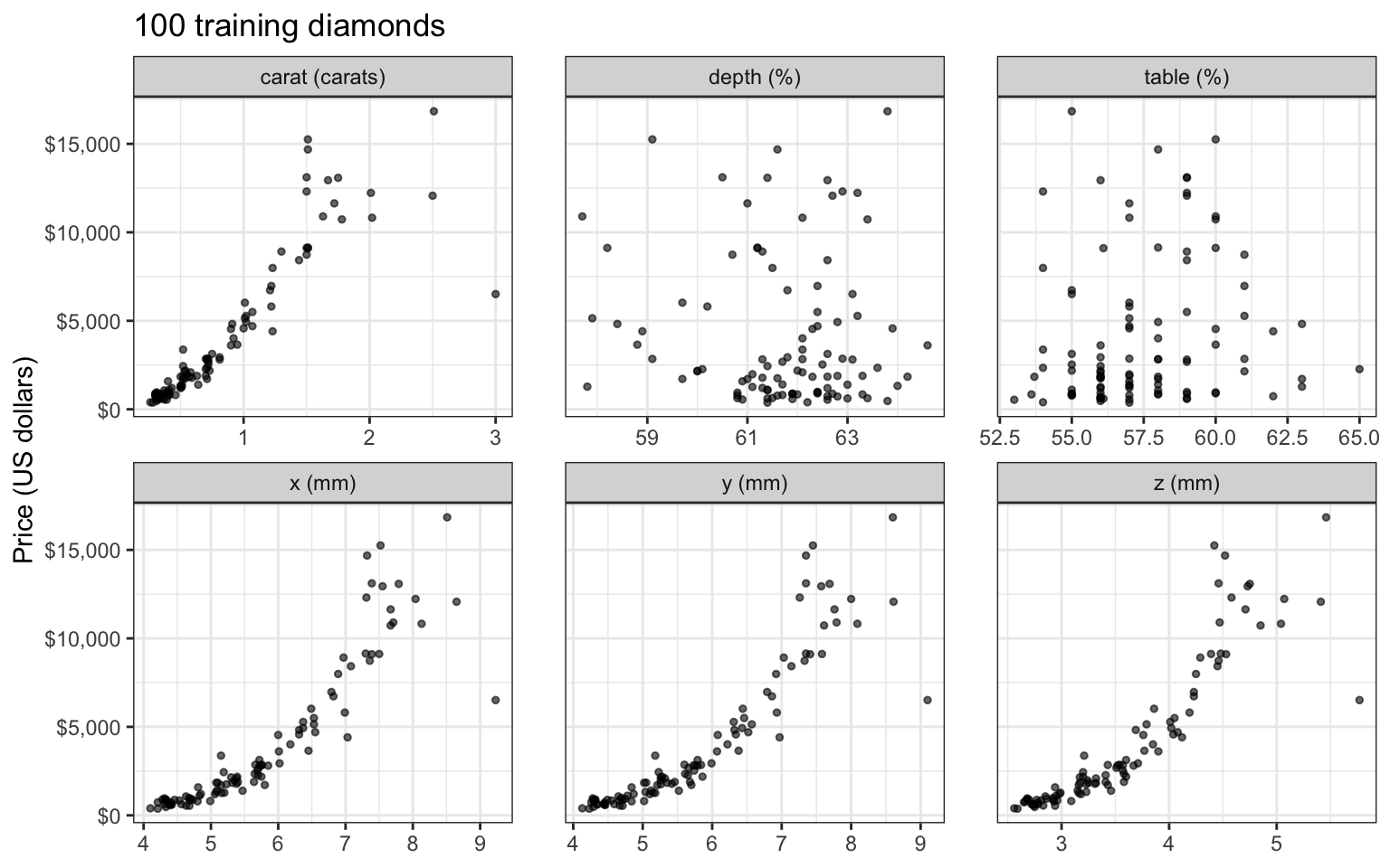

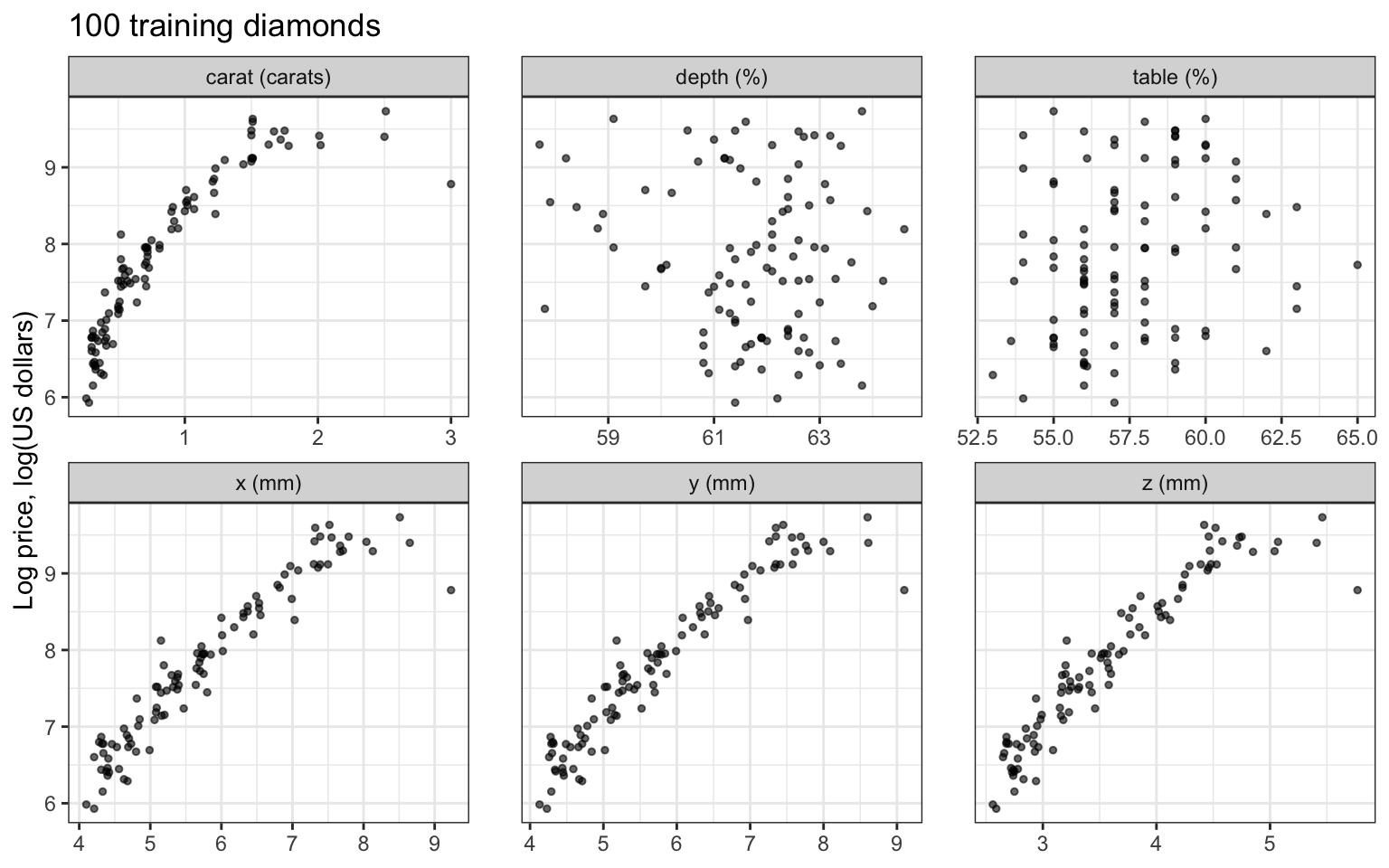
Price is right skewed: the mean training price, $4,096, is above the median, $2,226, and the most expensive training diamond costs 7.6 times the median. Price rises with carat and curves upward against the three dimensions, and its spread grows with size. Log price rises along a nearly straight line in x, y, and z, with a spread that does not grow, and bends against carat. Depth and table percentage show little relation to either response. The heaviest training diamond, at 3.00 carats, costs $6,512, far less than the other large diamonds.

The response is therefore the natural log of price, $y_i = \log\left(\texttt{price}_i\right)$, whose relationships with the dimensions are close to linear and whose spread is close to constant; every mean squared error below is in squared log dollars.

24.1.2 Least squares

# Mean squared error of predictions y_hat of responses y.
mse <- function(y, y_hat) {
  mean((y - y_hat)^2)
}

# Least squares on the six explanatory variables, fit to the training
# diamonds, and its training and test MSE.
ls_formula <- log_price ~ carat + depth + table + x + y + z
ls_fit <- lm(ls_formula, data = train)
y_train <- train$log_price
y_test <- test$log_price
ls_train_mse <- mse(y_train, fitted(ls_fit))
ls_test_pred <- predict(ls_fit, test)
ls_test_mse <- mse(y_test, ls_test_pred)

# The carat estimate and its standard error, and the correlation of carat
# with log price in the training diamonds.
ls_table <- summary(ls_fit)$coefficients
carat_cor <- cor(train$carat, y_train)

Least squares on the six explanatory variables has training MSE 0.0618 and test MSE 0.0726. Its carat estimate is −1.86 log dollars per carat, with standard error 0.24, although carat and log price have correlation 0.88 in the training diamonds. The estimate compares diamonds of equal x, y, and z: among those, the fit predicts the heavier ones to be cheaper. The principal components below separate that contrast from overall size.

As in the Ridge Regression lecture, the average variance of the least squares fitted values is $\sigma^2(p + 1)/n$. With $n = 100$ training diamonds it is 7% of the error variance; with all 53,917 diamonds it would be 0.013%, leaving a method that trades bias for variance little variance to remove.

24.2 Principal components regression

24.2.1 Scores and price

The principal components are computed as in the principal components lecture, but from the 100 training diamonds alone. The figure plots the log price of each training diamond against its score on each of the six components.

Code

# Standard deviation with divisor n.
sd_n <- function(v) {
  deviations <- v - mean(v)
  sqrt(mean(deviations^2))
}

# Standardize the columns of X with the given centers and scales.
standardize <- function(X, x_center, x_scale) {
  X_centered <- sweep(X, 2, x_center)
  sweep(X_centered, 2, x_scale, "/")
}

# Explanatory variables as matrices, and the standardized training features.
X_train <- as.matrix(train[features])
X_test <- as.matrix(test[features])
x_center <- colMeans(X_train)
x_scale <- apply(X_train, 2, sd_n)
X_std <- standardize(X_train, x_center, x_scale)

# Sign of the largest entry of phi in absolute value.
largest_sign <- function(phi) {
  largest <- which.max(abs(phi))
  sign(phi[largest])
}

# Loading vectors, signed as in the principal components lecture, their
# variances, and the n x p matrix of scores.
eig <- eigen(crossprod(X_std) / n_train, symmetric = TRUE)
flip <- apply(eig$vectors, 2, largest_sign)
Phi <- sweep(eig$vectors, 2, flip, "*")
dimnames(Phi) <- list(features, paste0("PC", 1:p))
v <- eig$values
Z <- X_std %*% Phi

# Proportion of variance explained, and correlation of log price with each
# component's scores.
pve <- v / p
score_cor <- drop(cor(y_train, Z))

# Loadings from all retained diamonds, signed the same way, and the largest
# difference from the training loadings over the first four components.
eig_all <- eigen(cor(kept[features]), symmetric = TRUE)
flip_all <- apply(eig_all$vectors, 2, largest_sign)
Phi_all <- sweep(eig_all$vectors, 2, flip_all, "*")
first_four <- 1:4
loading_gap <- max(abs(Phi[, first_four] - Phi_all[, first_four]))

# Log price against each component's scores, one panel each.
score_labels <- paste0("PC", 1:p,
                       ": PVE ", pct(pve, 2),
                       ", r = ", fmt_math(score_cor))
scores_plot <- as_tibble(Z, .name_repair = ~ score_labels) |>
  mutate(log_price = y_train) |>
  pivot_longer(-log_price, names_to = "component", values_to = "score") |>
  mutate(component = factor(component, levels = score_labels)) |>
  ggplot(aes(x = score, y = log_price)) +
  geom_point(alpha = 0.6, size = 1) +
  facet_wrap(~ component, scales = "free_x", nrow = 2) +
  labs(x = "Score",
       y = "Log price, log(US dollars)",
       title = title_train) +
  theme(panel.spacing.x = unit(1.5, "lines"))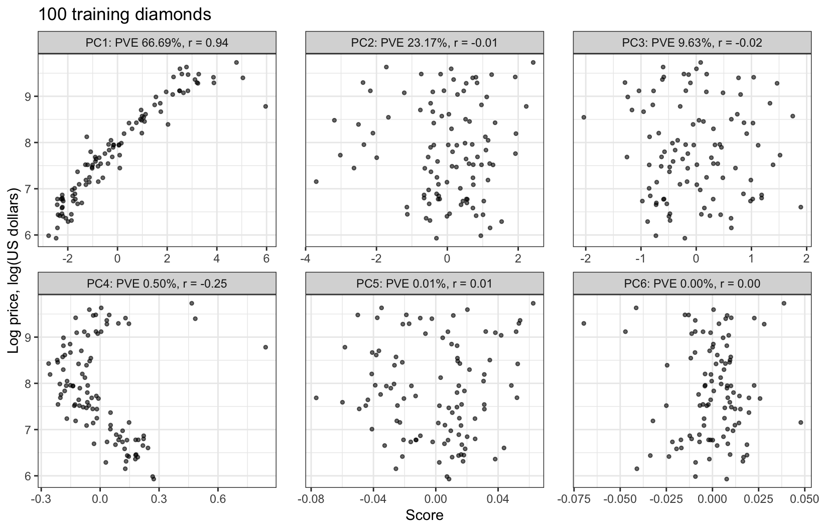

Log price rises along a nearly straight line in the first scores, correlation 0.937. The second and third components explain 32.8% of the variance of the features between them, and their scores are nearly uncorrelated with log price (−0.013 and −0.022). The fourth explains 0.50%, and its scores have correlation −0.249; the last two are flat. The training loadings of the first 4 components are within 0.06 of those computed from all 53,917 diamonds, so the components keep the interpretations of the principal components lecture: PC1 is size, PC2 and PC3 combine depth and table percentage, and PC4 contrasts weight with the three dimensions, with carat loading 0.87.

24.2.2 Model

Principal components regression fits the linear model

\[y_i = \theta_0 + \sum_{m=1}^M\theta_m z_{im} + \epsilon_i, \qquad \epsilon_i \stackrel{ind}{\sim} N\left(0, \sigma^2\right),\]

by least squares, where

$y_i$ is the log price of training diamond $i = 1, \ldots, n$, with $n = 100$,
$z_{im} = \tilde x_i\phi_m = \sum_{j=1}^p\phi_{jm}\tilde x_{ij}$ is its score on the $m$th principal component of the training features, with loading vector $\phi_m$ and variance $v_m$ over the training diamonds,
$\tilde x_{ij} = \left(x_{ij} - \bar x_j\right)/s_j$ is feature $j$ of diamond $i$: explanatory variable $j = 1, \ldots, p$, in the order carat, depth, table, x, y, and z, standardized with its mean $\bar x_j$ and standard deviation $s_j = \sqrt{\frac{1}{n}\sum_{i=1}^n\left(x_{ij} - \bar x_j\right)^2}$ over the training diamonds, so $p = 6$; $\tilde{\mathbf{X}}$ is the $n \times p$ matrix of features, with row $\tilde x_i$,
$M \in \{0, 1, \ldots, p\}$ is the number of components kept; $M = 0$, with no scores, is the null model,
$\theta_0, \theta_1, \ldots, \theta_M$ are the coefficients, and $\theta = \left(\theta_1, \ldots, \theta_M\right)^\top$, and
$\epsilon_i$ is the error, with variance $\sigma^2$.

A test diamond is standardized with the training means and standard deviations and projected on the training loading vectors, as a new diamond would be.

Write $z_m$ for the $n$-vector of scores on component $m$ and $\mathbf{Z}_M$ for the $n \times M$ matrix with columns $z_1, \ldots, z_M$. The scores have mean 0 and are uncorrelated, so $\mathbf{1}^\top\mathbf{Z}_M = 0$ and $\mathbf{Z}_M^\top\mathbf{Z}_M = n\,\text{diag}\left(v_1, \ldots, v_M\right)$. The normal equations then separate:

\[\hat\theta_0 = \bar y, \qquad \hat\theta_m = \frac{z_m^\top\left(y - \bar y\mathbf{1}\right)}{z_m^\top z_m} = \frac{z_m^\top\left(y - \bar y\mathbf{1}\right)}{nv_m}, \quad m = 1, \ldots, M.\]

Each $\hat\theta_m$ is the estimate of the simple linear regression of $y$ on $z_m$ alone, so keeping one more component leaves the earlier estimates unchanged. The fitted values are $\hat y_i = \bar y + \sum_{m=1}^M\hat\theta_m z_{im}$.

Treat the features as fixed and suppose the linear model in all $p$ features is correct, so that $E\left[y\right] = \theta_0\mathbf{1} + \sum_{m=1}^p\theta_m z_m$ for some $\theta_m$ and $Var\left[y\right] = \sigma^2\mathbf{I}_n$, writing the response vector $y$ in lowercase as the ridge lecture does. Since $z_m^\top\mathbf{1} = 0$, $\hat\theta_m = z_m^\top y/(nv_m)$, with

\[E\left[\hat\theta_m\right] = \theta_m, \qquad Var\left[\hat\theta_m\right] = \frac{z_m^\top z_m\,\sigma^2}{\left(nv_m\right)^2} = \frac{\sigma^2}{nv_m}.\]

Code

# Estimates on the scores, from the formula and from lm().
y_centered <- y_train - mean(y_train)
theta_hat <- drop(crossprod(Z, y_centered)) / (n_train * v)
scores_fit <- lm(y_train ~ Z)
theta_diff <- max(abs(coef(scores_fit)[-1] - theta_hat))

# Standard errors sigma_hat / sqrt(n v_m), sigma_hat from all p components.
sigma_hat <- sigma(scores_fit)
theta_se <- sigma_hat / sqrt(n_train * v)
theta_ratio <- abs(theta_hat) / theta_se

# The last component whose estimate is at least one standard error from
# zero, and the earlier ones that are not.
last_large <- max(which(theta_ratio >= 1))
small_before <- which(theta_ratio[seq_len(last_large)] < 1)

# Table of the variances, estimates, and standard errors.
theta_tibble <- tibble(Component = paste0("PC", 1:p),
                       v = fmt(v, 4),
                       theta = fmt(theta_hat, 3),
                       se = fmt(theta_se, 3),
                       ratio = fmt(theta_ratio, 1))
theta_columns <- c("Component",
                   "Variance $v_m$",
                   "Estimate $\\hat\\theta_m$",
                   "Standard error",
                   "$\\lvert\\hat\\theta_m\\rvert$ / standard error")
theta_table <- knitr::kable(theta_tibble,
                            col.names = theta_columns,
                            align = "lrrrr")

The table gives, for each component of the training features, its variance, the estimate $\hat\theta_m$, and the standard error $\hat\sigma/\sqrt{nv_m}$, with $\hat\sigma = 0.258$ from the fit on all 6 components. (lm() on the six columns of scores gives the same estimates, to within $1.6 \times 10^{-12}$.)

Component	Variance $v_m$	Estimate $\hat\theta_m$	Standard error	$\lvert\hat\theta_m\rvert$ / standard error
PC1	4.0012	0.479	0.013	37.1
PC2	1.3899	−0.011	0.022	0.5
PC3	0.5779	−0.029	0.034	0.9
PC4	0.0298	−1.474	0.149	9.9
PC5	0.0009	0.235	0.873	0.3
PC6	0.0003	−0.133	1.518	0.1

The intercept estimate, $\hat\theta_0 = \bar y = 7.82$ log dollars, is the predicted log price of a diamond with every score 0, one at the training means of all six explanatory variables, a price of $2,487. The standard error of $\hat\theta_6$ is 118 times that of $\hat\theta_1$, the square root of $v_1/v_6$. The estimates for PC5 and PC6 are 0.3 and 0.1 standard errors from zero, and the estimate for PC4, −1.47, is 10 standard errors from zero: one standard deviation of PC4 scores, 0.17, lowers the predicted log price by 0.25. A diamond heavier than its dimensions suggest is predicted to be cheaper.

24.2.3 Dropped components

Dropping components $M + 1, \ldots, p$ sets their estimates to zero. Under the same assumptions, with the features fixed, the mean squared error of the fitted values about the true mean at the training diamonds is

\[\frac{1}{n}E\left[\sum_{i=1}^n\left(\hat y_i - \theta_0 - \sum_{m=1}^p\theta_m z_{im}\right)^2\right] = \frac{\sigma^2}{n} + \sum_{m=1}^M\frac{\sigma^2}{n} + \sum_{m=M+1}^p\theta_m^2v_m.\]

This is the error in estimating the mean. The expected squared error in predicting a new response at the same features adds $\sigma^2$, which no choice of $M$ changes.

The scores of different components are orthogonal, so this mean squared error splits into one term for $\bar y$ and one per component. A kept component contributes the variance of $\hat\theta_mz_m$, which is $\frac{1}{n}z_m^\top z_m\,Var\left[\hat\theta_m\right] = \sigma^2/n$. A dropped component contributes its squared bias, $\frac{1}{n}\theta_m^2z_m^\top z_m = \theta_m^2v_m$. Dropping component $m$ therefore lowers the mean squared error of the fitted values exactly when $\theta_m^2v_m < \sigma^2/n$, that is, when $\left|\theta_m\right|$ is less than the standard error $\sigma/\sqrt{nv_m}$ of its estimate. Components with small $v_m$ have large standard errors, so they are the ones most likely to be worth dropping. PCR drops them in order of variance, last first, and cannot drop a component while keeping a later one.

Applied with the estimates in place of $\theta_m$, the rule is only a rough guide: on average $\hat\theta_m^2$ overstates $\theta_m^2$, since $E\left[\hat\theta_m^2\right] = \theta_m^2 + Var\left[\hat\theta_m\right]$. With that caveat, the last column of the table is below 1 for PC2, PC3, PC5, and PC6, so their terms look worth dropping. But PCR can drop only the components after the last one it keeps: keeping PC4 means keeping PC2 and PC3 as well.

24.2.4 Standardized-scale estimates

Substituting $z_{im} = \sum_{j=1}^p\phi_{jm}\tilde x_{ij}$ into the fitted values,

\[\hat y_i = \bar y + \sum_{m=1}^M\hat\theta_m\sum_{j=1}^p\phi_{jm}\tilde x_{ij} = \bar y + \sum_{j=1}^p\hat\beta_j\tilde x_{ij}, \qquad \hat\beta = \boldsymbol{\Phi}_M\hat\theta,\]

where

$\boldsymbol{\Phi}_M$ is the $p \times M$ matrix with columns $\phi_1, \ldots, \phi_M$, and
$\hat\beta = \left(\hat\beta_1, \ldots, \hat\beta_p\right)^\top$ are the PCR estimates on the standardized scale, $\hat\beta_j = \sum_{m=1}^M\phi_{jm}\hat\theta_m$; the estimate on the original scale is $\hat\beta_j/s_j$, as in the Ridge Regression lecture.

PCR is therefore a linear model in the $p$ standardized features, fit under a constraint: its estimate must lie in the span of the first $M$ loading vectors. Three consequences follow.

$M = p$ is least squares. $\boldsymbol{\Phi}$ is $p \times p$ and orthogonal, so $\mathbf{Z}_p = \tilde{\mathbf{X}}\boldsymbol{\Phi}$ has the same column space as $\tilde{\mathbf{X}}$, and least squares on the scores gives the same fitted values as least squares on the features.
$M$ is the tuning parameter. $M = 0$ is the null model, which predicts $\bar y$, and $M = p$ is least squares, the roles that $\lambda \to \infty$ and $\lambda = 0$ play in ridge regression.
PCR is not variable selection. Every loading is nonzero, so every $\hat\beta_j$ is in general nonzero, whatever $M$ is; predicting a new diamond needs all six explanatory variables.

24.2.5 Estimate path

Code

# Standardized-scale estimates for M = 1, ..., p: cumulative sums of
# theta_m phi_m, one column per M.
terms <- sweep(Phi, 2, theta_hat, "*")
B_std <- t(apply(terms, 1, cumsum))
colnames(B_std) <- 1:p

# Least squares on the standardized scale, and its largest difference from
# PCR with M = p.
b_ls_std <- coef(ls_fit)[features] * x_scale
ls_gap <- max(abs(B_std[, p] - b_ls_std))

# One row per feature and M, with M = 0 the null model.
path_data <- as_tibble(cbind(`0` = 0, B_std), rownames = "feature") |>
  pivot_longer(-feature, names_to = "M", values_to = "estimate") |>
  mutate(M = as.integer(M),
         feature = factor(feature, levels = features))

# Each standardized estimate against M.
path_plot <- ggplot(path_data,
                    aes(x = M,
                        y = estimate,
                        color = feature,
                        linetype = feature,
                        shape = feature)) +
  geom_hline(yintercept = 0, color = "grey50") +
  geom_line() +
  geom_point(size = 2) +
  scale_color_manual(values = okabe_ito) +
  scale_x_continuous(breaks = 0:p) +
  labs(x = "Number of components M",
       y = "Standardized estimate\n(log dollars per standard deviation)",
       color = NULL,
       linetype = NULL,
       shape = NULL,
       title = paste("PCR estimate path,", title_train)) +
  theme(legend.position = "bottom")

# The first M at which the carat estimate is negative, and the size
# features' estimates at the M before it.
size_vars <- c("carat", "x", "y", "z")
M_turn <- which(B_std["carat", ] < 0)[1]
size_before <- B_std[size_vars, M_turn - 1]
smallest_estimate <- min(abs(B_std))

The figure plots each standardized estimate $\hat\beta_j$ against $M$, from the null model at $M = 0$ to least squares at $M = p$.

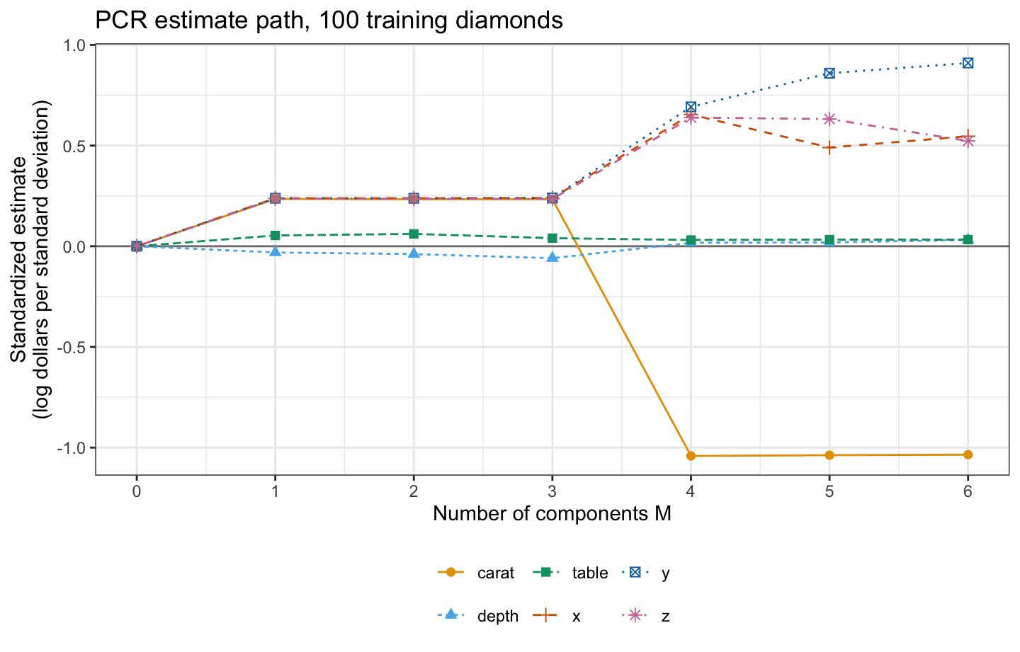
Up to $M = 3$ the four size features have nearly equal estimates, 0.234 to 0.240: the first component spreads the effect of size evenly over them, and PC2 and PC3 barely change it. At $M = 4$ the carat estimate turns negative, to −1.04, and the estimates for x, y, and z rise: PC4 separates weight from the dimensions. At $M = p$ the estimates are those of least squares, to within $1.3 \times 10^{-12}$. No estimate is zero at any $M \ge 1$; the smallest in absolute value is 0.017.

24.2.6 Shrinkage factors

Ridge regression also acts on the principal components. With the standardized features and the criterion $RSS + \lambda\sum_{j=1}^p\beta_j^2$ of the ridge lecture, $\tilde{\mathbf{X}}^\top\tilde{\mathbf{X}} = n\mathbf{R} = \boldsymbol{\Phi}\,\text{diag}\left(nv_1, \ldots, nv_p\right)\boldsymbol{\Phi}^\top$, so

\[\left(\tilde{\mathbf{X}}^\top\tilde{\mathbf{X}} + \lambda\mathbf{I}_p\right)^{-1} = \boldsymbol{\Phi}\,\text{diag}\left(\frac{1}{nv_1 + \lambda}, \ldots, \frac{1}{nv_p + \lambda}\right)\boldsymbol{\Phi}^\top.\]

With $\tilde{\mathbf{X}}\boldsymbol{\Phi} = \mathbf{Z}_p$ and $z_m^\top\left(y - \bar y\mathbf{1}\right) = nv_m\hat\theta_m$, the ridge fitted values are

\[\hat y^R_\lambda = \bar y\mathbf{1} + \tilde{\mathbf{X}}\left(\tilde{\mathbf{X}}^\top\tilde{\mathbf{X}} + \lambda\mathbf{I}_p\right)^{-1}\tilde{\mathbf{X}}^\top\left(y - \bar y\mathbf{1}\right) = \bar y\mathbf{1} + \sum_{m=1}^p\frac{z_mz_m^\top\left(y - \bar y\mathbf{1}\right)}{nv_m + \lambda} = \bar y\mathbf{1} + \sum_{m=1}^p\frac{v_m}{v_m + \lambda/n}\,\hat\theta_mz_m.\]

Ridge regression keeps every component and multiplies its least squares term $\hat\theta_mz_m$ by $v_m/(v_m + \lambda/n)$, a factor between 0 and 1 that is smallest for the components with the least variance. PCR multiplies the terms of the first $M$ components by 1 and the rest by 0, keeping or dropping each component as subset selection keeps or drops each feature.

Code

# Ridge estimate on the standardized scale from the closed form, at one
# lambda, and from the factors on the components.
lambda_check <- 10
lhs <- crossprod(X_std) + lambda_check * diag(p)
b_ridge_closed <- drop(solve(lhs, crossprod(X_std, y_centered)))
ridge_factor <- function(lambda) {
  v / (v + lambda / n_train)
}
factor_terms <- ridge_factor(lambda_check) * theta_hat
b_ridge_factors <- drop(Phi %*% factor_terms)
factor_gap <- max(abs(b_ridge_closed - b_ridge_factors))

# Factors of PCR with M = 4 and of ridge regression at three lambdas.
M_show <- 4
lambda_show <- c(1, 10, 100)
method_labels <- c(paste0("PCR, M = ", M_show),
                   paste0("Ridge, lambda = ", lambda_show))
method_math <- c(paste0("'PCR, '*M == ", M_show),
                 paste0("'Ridge, '*lambda == ", lambda_show))
method_legend <- parse(text = method_math)
pcr_factor <- as.numeric(1:p <= M_show)
ridge_factors <- map(lambda_show, ridge_factor) |>
  unlist()
factor_data <- tibble(method = rep(method_labels, each = p),
                      m = rep(1:p, length(method_labels)),
                      factor = c(pcr_factor, ridge_factors)) |>
  mutate(method = factor(method, levels = method_labels))

# The factor of each component against m.
factor_plot <- ggplot(factor_data,
                      aes(x = m,
                          y = factor,
                          color = method,
                          linetype = method,
                          shape = method)) +
  geom_line() +
  geom_point(size = 2.5) +
  scale_color_manual(values = okabe_ito[c(4, 5, 3, 1)],
                     labels = method_legend) +
  scale_linetype_discrete(labels = method_legend) +
  scale_shape_discrete(labels = method_legend) +
  scale_x_continuous(breaks = 1:p, labels = paste0("PC", 1:p)) +
  labs(x = "Component",
       y = "Factor on the component's term",
       color = NULL,
       linetype = NULL,
       shape = NULL,
       title = title_train) +
  theme(legend.position = "bottom")

The ridge estimate from the closed form at $\lambda = 10$ and $\boldsymbol{\Phi}$ times the shrunken $\hat\theta_m$ agree to within $3.8 \times 10^{-15}$. The figure plots the factor on each component’s term for PCR with $M = 4$ and for ridge regression at three values of $\lambda$.

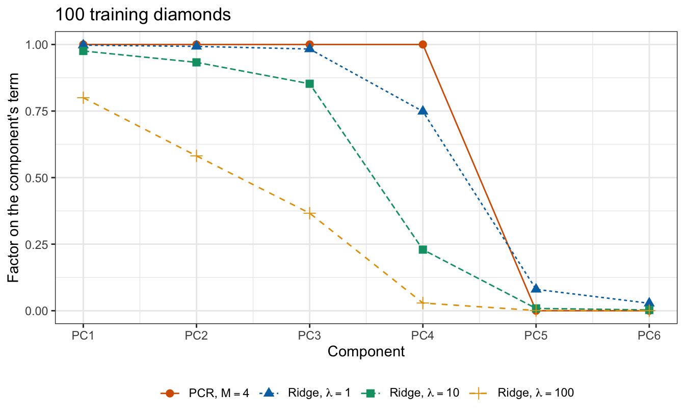
At $\lambda = 10$ the PC4 term keeps 23% of its least squares size, where PCR with $M = 4$ keeps all of it, while PCR keeps the PC2 and PC3 terms in full although their estimates are small.

24.2.7 pcr()

The function pcr_path() computes the PCR estimates on the original scale for every $M$ at once; path_estimates() turns any set of directions and estimates into original-scale estimates, and is reused for PLS below.

# Original-scale estimates for M = 1, ..., p, one column each, from the
# directions (columns of R_dir, whose scores are the standardized features
# times R_dir), the estimates theta, and the standardization.
path_estimates <- function(R_dir, theta, x_center, x_scale, y_bar) {
  # Standardized-scale estimates: cumulative sums of theta_m times r_m.
  terms <- sweep(R_dir, 2, theta, "*")
  b_std <- t(apply(terms, 1, cumsum))

  # Back to the original scale.
  b <- b_std / x_scale
  intercept <- y_bar - colSums(b * x_center)
  rbind(`(Intercept)` = intercept, b)
}

# PCR estimates on the original scale for M = 1, ..., p.
pcr_path <- function(X, y) {
  # Standardize with the means and standard deviations of these data.
  x_center <- colMeans(X)
  x_scale <- apply(X, 2, sd_n)
  X_std <- standardize(X, x_center, x_scale)

  # Loading vectors and scores.
  eig <- eigen(crossprod(X_std) / nrow(X), symmetric = TRUE)
  Z <- X_std %*% eig$vectors

  # Simple regression of the centered response on each column of scores.
  y_centered <- y - mean(y)
  theta <- drop(crossprod(Z, y_centered)) / colSums(Z^2)

  path_estimates(eig$vectors, theta, x_center, x_scale, mean(y))
}

pls::pcr() fits the same model. With scale = TRUE it standardizes with divisor $n - 1$, which divides every feature by the same extra factor and changes no fit, and its coef() reports estimates for its own standardized features, so the check compares predictions.

# PCR by hand and by pcr(), both fit to the training diamonds.
B_pcr <- pcr_path(X_train, y_train)
pcr_fit <- pcr(ls_formula, ncomp = p, data = train, scale = TRUE)

# Predictions of the test diamonds for every M, and the largest difference.
pcr_pred_hand <- cbind(1, X_test) %*% B_pcr
pcr_pred_pls <- predict(pcr_fit, test, ncomp = 1:p)[, 1, ]
pcr_check <- max(abs(pcr_pred_hand - pcr_pred_pls))

Over the 53,817 test diamonds and the 6 values of $M$, the two sets of predictions differ by at most $5.3 \times 10^{-12}$ log dollars.

24.2.8 Components kept

$M$ is chosen by 10-fold cross-validation on the training diamonds, using the fold assignment fold_id that the split chunk drew along with the training sample. The $k$-fold cross-validation estimate $\text{CV}_{(k)}(M)$, with $k = 10$, is the mean squared error of the predictions of the held-out folds. The standardization and the principal components are computed from the data the model is fit to, so in each fold they are recomputed from the training folds only; the held-out fold is standardized with the training folds’ means and standard deviations and projected on their loading vectors. pcr_path() does all of this when it is given the training folds.

# Sums of squared errors of the held-out fold l for M = 1, ..., p, from the
# estimates that path() computes from the training folds.
fold_sse <- function(l, path) {
  out <- fold_id == l
  B <- path(X_train[!out, ], y_train[!out])
  y_hat <- cbind(1, X_train[out, ]) %*% B
  colSums((y_train[out] - y_hat)^2)
}

# Cross-validation estimate for M = 1, ..., p.
cv_estimate <- function(path) {
  sse <- sapply(seq_len(n_folds), fold_sse, path = path)
  rowSums(sse) / n_train
}

# PCR, and the M with the smallest estimate.
cv_pcr <- cv_estimate(pcr_path)
M_pcr <- which.min(cv_pcr)

# pcr()'s own cross-validation on the same folds.
segments <- split(seq_len(n_train), fold_id)
pcr_cv_fit <- pcr(ls_formula,
                  ncomp = p,
                  data = train,
                  scale = TRUE,
                  validation = "CV",
                  segments = segments)
cv_pcr_pls <- MSEP(pcr_cv_fit, estimate = "CV", intercept = FALSE)$val[1, 1, ]
cv_pcr_check <- max(abs(cv_pcr - cv_pcr_pls))

Code

# Null model: the mean of the training folds predicts the held-out fold.
null_sse <- function(l) {
  out <- fold_id == l
  sum((y_train[out] - mean(y_train[!out]))^2)
}
null_fold_sse <- map_dbl(seq_len(n_folds), null_sse)
cv_null <- sum(null_fold_sse) / n_train

# Cross-validation of the regression on the first M columns of scores Z_all,
# computed once from all the training diamonds: held-out fold l.
outside_sse <- function(l, Z_all) {
  out <- fold_id == l
  sse <- numeric(p)
  for (M in seq_len(p)) {
    Z_in <- cbind(1, Z_all[!out, seq_len(M)])
    Z_out <- cbind(1, Z_all[out, seq_len(M)])
    b <- qr.solve(Z_in, y_train[!out])
    sse[M] <- sum((y_train[out] - Z_out %*% b)^2)
  }
  sse
}

# The same for all folds, for M = 1, ..., p.
outside_cv <- function(Z_all) {
  sse <- sapply(seq_len(n_folds), outside_sse, Z_all = Z_all)
  rowSums(sse) / n_train
}

# PCR with the components computed once from all the training diamonds.
cv_pcr_outside <- outside_cv(Z)
pcr_outside_gap <- max(abs(cv_pcr_outside - cv_pcr))

# The estimate against M, with the chosen M and least squares labeled.
cv_axis_label <- paste0(n_folds, "-fold CV estimate of test MSE")
pcr_cv_data <- tibble(M = 1:p, cv = cv_pcr)
pcr_cv_plot <- ggplot(pcr_cv_data, aes(x = M, y = cv)) +
  geom_line() +
  geom_point(size = 2) +
  annotate("point",
           x = M_pcr,
           y = cv_pcr[M_pcr],
           size = 4,
           shape = 1,
           color = "#D55E00") +
  annotate("text",
           x = M_pcr,
           y = cv_pcr[M_pcr],
           label = paste("Chosen, M =", M_pcr),
           vjust = -1.5,
           color = "#D55E00") +
  annotate("text",
           x = p,
           y = cv_pcr[p],
           label = "Least squares, M = p",
           vjust = -1.5,
           hjust = 1) +
  scale_x_continuous(breaks = 1:p) +
  labs(x = "Number of components M",
       y = cv_axis_label,
       title = paste("PCR,", title_train))

The cross-validation estimates from pcr_path() and from pcr() with validation = "CV" and the same folds as segments agree to within $1.7 \times 10^{-15}$; pcr() also standardizes within each fold. The figure plots $\text{CV}_{(10)}(M)$ against $M$.

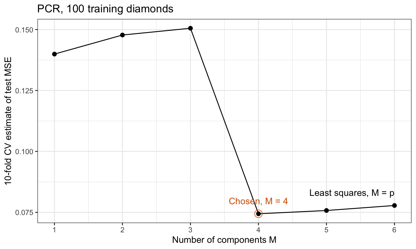
The estimate for the null model, $M = 0$, is 1.063. With one component it falls to 0.1399, and it rises with the second and third components, to 0.1505, which add a variance of $\sigma^2/n$ each to the fit but almost nothing to its mean. The fourth component halves it, to 0.0744. Beyond that the estimate rises again, to 0.0778 for least squares, and the smallest estimate is at $M = 4$.

Computing the standardization and the components once from all 100 training diamonds, and cross-validating only the regression on the scores, changes the estimate by at most 0.00103 over the 6 values of $M$. Principal components do not use the response, so the held-out fold’s log prices never helped choose the directions they are predicted with; for PLS, below, they would.

24.3 Partial least squares

24.3.1 Features and price

PCR chose its directions without the response: PC2 and PC3 explain 32.8% of the variance of the features and add 0.0006 to the training $R^2$ of log price, while PC4 explains 0.50% and adds 0.062. The figure plots log price against each standardized feature of the training diamonds, with the least squares line of each simple regression.

Code

# Simple regression estimate of log price on each standardized feature,
# which is also their sample covariance, since each feature has variance 1.
slopes <- drop(crossprod(X_std, y_centered)) / n_train

# Log price against each standardized feature, with its least squares line.
slope_labels <- paste0(features, ": slope ", fmt_math(slopes, 3))
slope_plot <- as_tibble(X_std, .name_repair = ~ slope_labels) |>
  mutate(log_price = y_train) |>
  pivot_longer(-log_price, names_to = "feature", values_to = "value") |>
  mutate(feature = factor(feature, levels = slope_labels)) |>
  ggplot(aes(x = value, y = log_price)) +
  geom_point(alpha = 0.6, size = 1) +
  geom_smooth(method = "lm",
              formula = y ~ x,
              se = FALSE,
              color = "#D55E00") +
  facet_wrap(~ feature, nrow = 2) +
  labs(x = "Standardized feature",
       y = "Log price, log(US dollars)",
       title = title_train)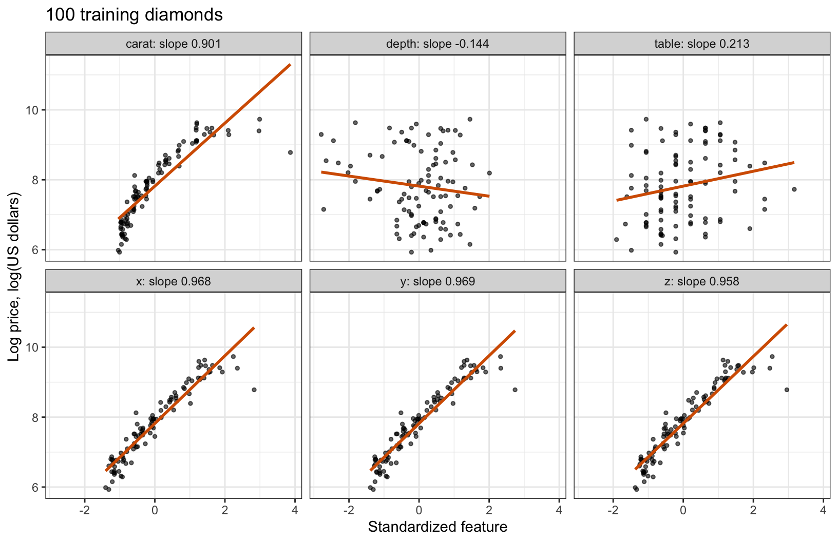

The four size features have slopes 0.901 to 0.969 log dollars per standard deviation, depth −0.144 and table 0.213. Each feature has mean 0 and variance 1, so its slope, $\frac{1}{n}\sum_i\tilde x_{ij}\left(y_i - \bar y\right)$, is also the sample covariance of the feature with log price.

24.3.2 First direction

Partial least squares chooses its first direction with these slopes. Its loadings are

\[\phi^{\text{PLS}}_{j1} = \frac{g_j}{\sqrt{\sum_{l=1}^p g_l^2}}, \qquad g_j = \frac{1}{n}\sum_{i=1}^n\tilde x_{ij}\left(y_i - \bar y\right),\]

with scores $z^{\text{PLS}}_{i1} = \sum_{j=1}^p\phi^{\text{PLS}}_{j1}\tilde x_{ij}$, where

$g_j$ is the simple regression estimate of $y$ on feature $j$, the slope in the figure, and $g = \left(g_1, \ldots, g_p\right)^\top = \tilde{\mathbf{X}}^\top\left(y - \bar y\mathbf{1}\right)/n$,
$\phi^{\text{PLS}}_1 = g/\left\|g\right\|$ is the first PLS direction, scaled to unit length like a loading vector (the scale changes $\hat\theta_1$ but no fitted value), and
$z^{\text{PLS}}_{i1}$ is the score of diamond $i$ on it.

The direction maximizes a criterion, as $\phi_1$ does. The scores of a unit vector $a$ have mean 0 and sample covariance with $y$

\[\frac{1}{n}\sum_{i=1}^n\tilde x_ia\left(y_i - \bar y\right) = a^\top g.\]

By the Cauchy-Schwarz inequality, $\left(a^\top g\right)^2 \le \left\|a\right\|^2\left\|g\right\|^2 = \left\|g\right\|^2$, with equality only at $a = \pm g/\left\|g\right\|$. So the first PLS direction is the unit vector whose scores have the largest squared covariance with the response, where the first principal component is the one whose scores have the largest variance. The squared covariance factors as

\[\left(a^\top g\right)^2 = R_a^2\,s_a^2\,s_y^2,\]

where

$R_a^2$ is the squared sample correlation of the scores $\tilde{\mathbf{X}}a$ with $y$, which is the $R^2$ of the simple regression of $y$ on them,
$s_a^2$ is the sample variance of the scores, and
$s_y^2$ is the sample variance of $y$, both with divisor $n$.

With $s_y^2$ fixed, PLS balances two goals. The first principal component maximizes $s_a^2$ alone. The least squares fitted values maximize $R_a^2$ alone: the simple regression of $y$ on $\tilde{\mathbf{X}}a$ is a model contained in the multiple regression on $\tilde{\mathbf{X}}$, so $R_a^2$ is at most the least squares $R^2$, attained by $a = \hat\beta^{\text{LS}}/\left\|\hat\beta^{\text{LS}}\right\|$, the least squares direction, with $\hat\beta^{\text{LS}}$ the least squares estimate on the standardized scale (PCR with $M = p$).

Code

# The first PLS direction and the least squares direction, unit length.
phi_pls_1 <- slopes / sqrt(sum(slopes^2))
a_ls <- b_ls_std / sqrt(sum(b_ls_std^2))

# Variance, squared correlation with log price, and squared covariance with
# log price of the scores of a unit vector a.
direction_summary <- function(a) {
  scores <- drop(X_std %*% a)
  c(variance = sd_n(scores)^2,
    cor2 = cor(scores, y_train)^2,
    cov2 = mean(scores * y_centered)^2)
}
direction_names <- c("First principal component",
                     "First PLS direction",
                     "Least squares direction")
directions <- cbind(Phi[, 1], phi_pls_1, a_ls)
summaries <- apply(directions, 2, direction_summary)
colnames(summaries) <- direction_names

# Table of the three criteria.
summary_tibble <- tibble(Direction = direction_names,
                         variance = fmt(summaries["variance", ], 3),
                         cor2 = fmt(summaries["cor2", ], 4),
                         cov2 = fmt(summaries["cov2", ], 4))
summary_columns <- c("Direction",
                     "Variance of scores",
                     "Squared correlation with log price",
                     "Squared covariance with log price")
summary_table <- knitr::kable(summary_tibble,
                              col.names = summary_columns,
                              align = "lrrr")

# The loadings of the three directions, feature by feature.
direction_data <- tibble(
  feature = factor(rep(features, 3), levels = rev(features)),
  loading = c(directions),
  direction = factor(rep(direction_names, each = p), levels = direction_names)
)
direction_plot <- ggplot(direction_data,
                         aes(x = loading,
                             y = feature,
                             color = direction,
                             shape = direction)) +
  geom_vline(xintercept = 0, color = "grey50") +
  geom_point(size = 2.5, position = position_dodge(width = 0.6)) +
  scale_color_manual(values = okabe_ito[c(5, 4, 3)]) +
  scale_shape_manual(values = c(16, 17, 15)) +
  guides(color = guide_legend(nrow = 2, byrow = TRUE),
         shape = guide_legend(nrow = 2, byrow = TRUE)) +
  labs(x = "Loading",
       y = NULL,
       color = NULL,
       shape = NULL,
       title = title_train) +
  theme(legend.position = "bottom")

# Largest difference between the first PLS direction and the first
# principal component.
pls_pc_gap <- max(abs(phi_pls_1 - Phi[, 1]))

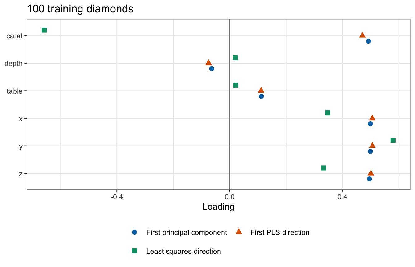
The figure plots the loadings of the first principal component, the first PLS direction, and the least squares direction, each of unit length, and the table gives the three criteria for each.

Direction	Variance of scores	Squared correlation with log price	Squared covariance with log price
First principal component	4.001	0.8781	3.6687
First PLS direction	3.999	0.8793	3.6712
Least squares direction	0.397	0.9408	0.3900

Each direction wins on its own criterion: the first principal component has the largest variance, 4.0012, the least squares direction the largest squared correlation, 0.9408, the training $R^2$ of least squares, and the first PLS direction the largest squared covariance, 3.6712. On these diamonds the first PLS direction and the first principal component nearly coincide, their loadings within 0.021 of each other, because the direction in which the features vary most, size, is also the one most related to log price. The least squares direction loads negatively on carat and has variance only 0.397: it leans on the contrast between weight and the dimensions that PC4 carries.

24.3.3 Later directions

The second PLS direction repeats the construction on what the first scores do not explain. Each feature is regressed on $z^{\text{PLS}}_1$ and replaced by its residuals,

\[\tilde{\mathbf{x}}^{(2)}_{\cdot j} = \tilde{\mathbf{x}}_{\cdot j} - \frac{\left(z^{\text{PLS}}_1\right)^\top\tilde{\mathbf{x}}_{\cdot j}}{\left(z^{\text{PLS}}_1\right)^\top z^{\text{PLS}}_1}\,z^{\text{PLS}}_1,\]

where

$\tilde{\mathbf{x}}_{\cdot j}$ is column $j$ of $\tilde{\mathbf{X}}$, the $n$-vector of feature $j$ over the training diamonds (bold, with a dot for the row index, to distinguish it from the row $\tilde x_i$ of one diamond), and
$\tilde{\mathbf{x}}^{(2)}_{\cdot j}$ is column $j$ of $\tilde{\mathbf{X}}^{(2)}$, the $n \times p$ matrix of residual features.

Then

\[\phi^{\text{PLS}}_2 \propto \left(\tilde{\mathbf{X}}^{(2)}\right)^\top\left(y - \bar y\mathbf{1}\right), \qquad z^{\text{PLS}}_2 = \tilde{\mathbf{X}}^{(2)}\phi^{\text{PLS}}_2,\]

with $\phi^{\text{PLS}}_2$ of unit length, and so on: direction $m$ uses the residuals $\tilde{\mathbf{X}}^{(m)}$ of the features after regressing them on the first $m - 1$ scores. Three properties make PLS a regression like PCR.

The scores are uncorrelated. Every column of $\tilde{\mathbf{X}}^{(m)}$ is orthogonal to $z^{\text{PLS}}_1, \ldots, z^{\text{PLS}}_{m-1}$, and so is $z^{\text{PLS}}_m$, a combination of those columns. As for PCR, the estimate $\hat\theta_m$ of the regression of $y$ on $M$ PLS scores is the simple regression estimate on $z^{\text{PLS}}_m$, and the fitted values are $\bar y + \sum_{m=1}^M\hat\theta_mz^{\text{PLS}}_{im}$. The orthogonality also means that $\phi^{\text{PLS}}_m$ is proportional to the covariances of the residual features with the residuals of $y$ from the first $m - 1$ scores.
PLS is a linear model in the features. Each $\tilde{\mathbf{X}}^{(m)}$ is $\tilde{\mathbf{X}}$ minus multiples of earlier scores, which are themselves combinations of the columns of $\tilde{\mathbf{X}}$, so $z^{\text{PLS}}_m = \tilde{\mathbf{X}}r_m$ for a $p$-vector $r_m$, with $r_1 = \phi^{\text{PLS}}_1$, and the standardized-scale estimate is $\hat\beta = \sum_{m=1}^M\hat\theta_mr_m$.
$M = p$ is least squares, when the $p$ scores span the column space of $\tilde{\mathbf{X}}$, as they do here.

pls_path() carries out these steps, and pls::plsr() fits the same model.

# PLS on the standardized features: the directions, the vectors r_m with
# scores X_std r_m, the estimates theta, and the standardization.
pls_directions <- function(X, y) {
  # Standardize the features; center the response.
  x_center <- colMeans(X)
  x_scale <- apply(X, 2, sd_n)
  X_std <- standardize(X, x_center, x_scale)
  y_centered <- y - mean(y)
  p <- ncol(X)

  # Directions, vectors r_m, and estimates, filled one direction at a time.
  W <- matrix(0, p, p)
  R_dir <- matrix(0, p, p)
  theta <- numeric(p)
  X_m <- X_std

  for (m in seq_len(p)) {
    # Direction: covariances of the residual features with the response,
    # scaled to unit length.
    g <- drop(crossprod(X_m, y_centered)) / nrow(X)
    W[, m] <- g / sqrt(sum(g^2))

    # Scores, and the simple regression of the response on them.
    z <- drop(X_m %*% W[, m])
    theta[m] <- sum(z * y_centered) / sum(z^2)

    # The scores as a combination of the standardized features: they lie in
    # the column space of X_std, so least squares recovers r_m exactly.
    R_dir[, m] <- qr.solve(X_std, z)

    # Replace each feature by its residuals from regressing it on z.
    feature_slopes <- drop(crossprod(X_m, z)) / sum(z^2)
    X_m <- X_m - z %o% feature_slopes
  }

  list(W = W,
       R_dir = R_dir,
       theta = theta,
       x_center = x_center,
       x_scale = x_scale,
       y_bar = mean(y))
}

# PLS estimates on the original scale for M = 1, ..., p.
pls_path <- function(X, y) {
  d <- pls_directions(X, y)
  path_estimates(d$R_dir, d$theta, d$x_center, d$x_scale, d$y_bar)
}

# PLS by hand and by plsr(), both fit to the training diamonds.
pls_d <- pls_directions(X_train, y_train)
B_pls <- pls_path(X_train, y_train)
pls_fit <- plsr(ls_formula, ncomp = p, data = train, scale = TRUE)

# Predictions of the test diamonds for every M, and the largest difference.
pls_pred_hand <- cbind(1, X_test) %*% B_pls
pls_pred_pls <- predict(pls_fit, test, ncomp = 1:p)[, 1, ]
pls_check <- max(abs(pls_pred_hand - pls_pred_pls))

# Directions: plsr() calls them loading weights.
pls_weights <- unclass(loading.weights(pls_fit))
weight_check <- max(abs(pls_weights - pls_d$W))

# PLS with M = p against least squares.
pls_ls_gap <- max(abs(B_pls[, p] - coef(ls_fit)))

The directions of pls_path() and the loading weights of plsr() agree to within $2.2 \times 10^{-11}$, and their predictions of the test diamonds for every $M$ to within $5.8 \times 10^{-13}$ log dollars. With $M = p$ the PLS estimates equal those of least squares to within $3.9 \times 10^{-12}$.

24.3.4 Directions compared

Code

# Scores of the PLS directions, their variances, and the largest correlation
# between two columns of them.
Z_pls <- X_std %*% pls_d$R_dir
v_pls <- apply(Z_pls, 2, sd_n)^2
pls_score_cors <- cor(Z_pls)[upper.tri(diag(p))]
max_pls_score_cor <- max(abs(pls_score_cors))
pls_cor <- drop(cor(y_train, Z_pls))

# Training R^2 of the fit on the first M directions.
train_r2 <- function(B) {
  y_hat <- cbind(1, X_train) %*% B
  residual_ms <- colMeans((y_train - y_hat)^2)
  1 - residual_ms / mean(y_centered^2)
}
r2_pcr <- train_r2(B_pcr)
r2_pls <- train_r2(B_pls)

# One row per method and m.
method_levels <- c("PCR", "PLS")
compare_data <- tibble(method = factor(rep(method_levels, each = p),
                                       levels = method_levels),
                       m = rep(1:p, 2),
                       variance = c(v, v_pls),
                       r2 = c(r2_pcr, r2_pls))

# Shared look of the two tabs.
compare_layers <- list(
  geom_line(),
  geom_point(size = 2.5),
  scale_color_manual(values = okabe_ito[c(5, 4)]),
  scale_x_continuous(breaks = 1:p),
  labs(color = NULL, linetype = NULL, shape = NULL, title = title_train),
  theme(legend.position = "bottom")
)
compare_aes <- aes(color = method, linetype = method, shape = method)

# Variance of the m-th scores, on a log scale.
variance_plot <- ggplot(compare_data, aes(x = m, y = variance)) +
  compare_aes +
  compare_layers +
  scale_y_log10() +
  labs(x = "Direction m",
       y = "Variance of the m-th scores (log scale)")

# Training R^2 of the first M directions.
r2_plot <- ggplot(compare_data, aes(x = m, y = r2)) +
  compare_aes +
  compare_layers +
  labs(x = "Number of directions M",
       y = expression("Training " * R^2))

# PLS fits the training diamonds at least as well at every M < p.
pls_fits_better <- all(r2_pls[-p] >= r2_pcr[-p])

The tabs compare the PLS directions with the principal components of the training features: the variance of the scores on each direction, and the training $R^2$ of the regression of log price on the first $M$ directions.

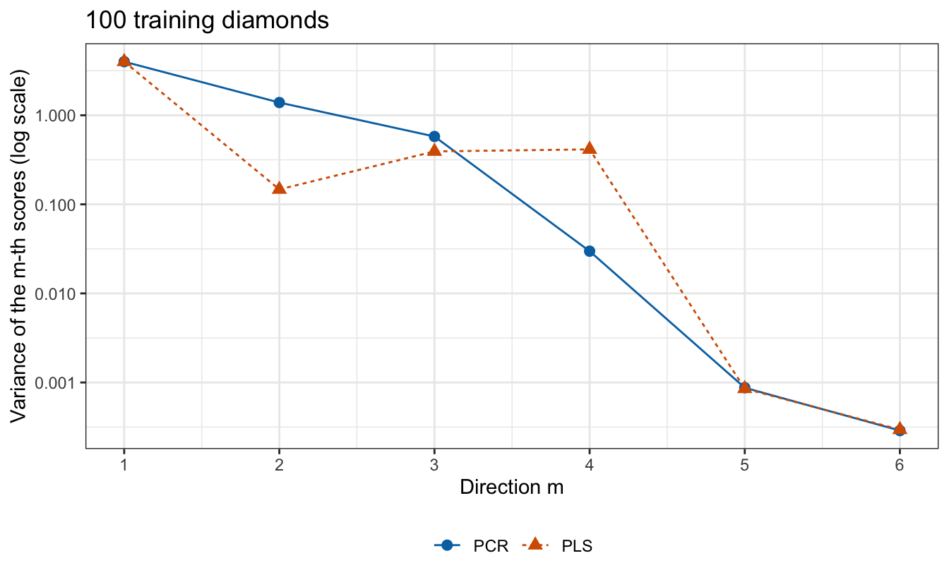
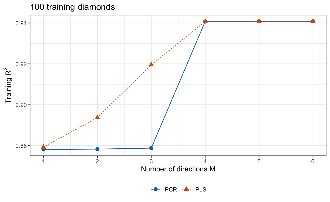
The principal component variances fall by construction. The PLS variances do not: the second PLS direction has variance 0.147, against 1.390 for PC2, and the third and fourth are larger than the second, 0.393 and 0.414. PLS scores are uncorrelated too, the largest correlation between two columns being $1.3 \times 10^{-14}$, and the squared correlations of log price with the second to fourth PLS scores, 0.014, 0.026, and 0.021, are larger than those with PC2 and PC3. So the training $R^2$ of PLS rises with each of the first four directions, from 0.879 to 0.941, while that of PCR stays near 0.878 until PC4 lifts it to 0.941. PLS fits the training diamonds at least as well as PCR at every $M < p$, and both reach the least squares fit at $M = p$.

24.3.5 Directions kept

PLS directions use the response, so they too are recomputed from the training folds in each fold. cv_estimate(pls_path) does this on the same folds.

# PLS cross-validated on the same folds, and the M with the smallest
# estimate.
cv_pls <- cv_estimate(pls_path)
M_pls <- which.min(cv_pls)

# plsr()'s own cross-validation on the same folds.
pls_cv_fit <- plsr(ls_formula,
                   ncomp = p,
                   data = train,
                   scale = TRUE,
                   validation = "CV",
                   segments = segments)
cv_pls_pls <- MSEP(pls_cv_fit, estimate = "CV", intercept = FALSE)$val[1, 1, ]
cv_pls_check <- max(abs(cv_pls - cv_pls_pls))

Code

# PLS with the directions computed once from all the training diamonds, and
# how much smaller its estimate is.
cv_pls_outside <- outside_cv(Z_pls)
pls_optimism <- cv_pls - cv_pls_outside
M_optimism <- which.max(pls_optimism)
M_pls_outside <- which.min(cv_pls_outside)

# The M at which the PCR estimate exceeds the PLS estimate the most.
M_gap <- which.max(cv_pcr - cv_pls)

# Both curves, with the chosen M of each circled.
cv_data <- tibble(method = factor(rep(method_levels, each = p),
                                  levels = method_levels),
                  M = rep(1:p, 2),
                  cv = c(cv_pcr, cv_pls))
chosen_data <- tibble(method = factor(method_levels, levels = method_levels),
                      M = c(M_pcr, M_pls),
                      cv = c(cv_pcr[M_pcr], cv_pls[M_pls]))
cv_plot <- ggplot(cv_data,
                  aes(x = M,
                      y = cv,
                      color = method,
                      linetype = method,
                      shape = method)) +
  geom_line() +
  geom_point(size = 2.5) +
  geom_point(data = chosen_data,
             size = 5,
             shape = 1,
             show.legend = FALSE) +
  scale_color_manual(values = okabe_ito[c(5, 4)]) +
  scale_x_continuous(breaks = 1:p) +
  labs(x = "Number of directions M",
       y = cv_axis_label,
       color = NULL,
       linetype = NULL,
       shape = NULL,
       title = title_train,
       caption = "Circles: the chosen M of each method.") +
  theme(legend.position = "bottom")

The estimates from pls_path() and from plsr() with the same folds agree to within $3.4 \times 10^{-15}$. The figure plots $\text{CV}_{(10)}(M)$ for PCR and PLS.

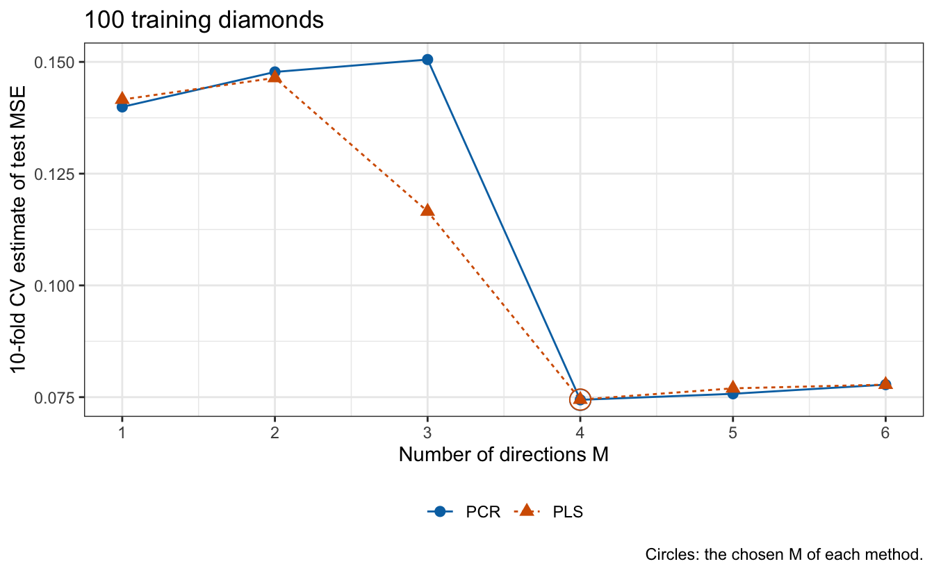
At $M = 3$, where the two curves differ most, the PLS estimate is 0.1165, against 0.1505 for PCR, because the PLS directions after the first carry part of what PC4 adds. PLS reaches its smallest estimate, 0.0745, at $M = 4$, and PCR its smallest, 0.0744, at $M = 4$, both below the least squares estimate of 0.0778.

Computing the PLS directions once from all 100 training diamonds, and cross-validating only the regression on their scores, lowers the estimate by as much as 0.0160, at $M = 3$ (14% of the estimate there), against at most 0.00103 for PCR. The log prices of each held-out fold then helped choose the directions they are predicted with, so the estimate is optimistic. The size of the optimism depends on $M$: at the chosen $M = 4$ it is only 0.0001, and the estimates computed outside the folds would choose $M = 4$, the same value.

24.3.6 Bias and variance

The PLS directions are chosen to covary with the response, and on these diamonds they fit the training diamonds at least as well as the principal components at every $M < p$. Choosing directions this way can lower the bias of a fit with $M$ directions, but training fit alone cannot distinguish that from fitting noise; because the directions depend on the training responses, the fit can also have more variance than PCR’s, whose directions depend only on the features. Neither method can improve much on least squares when least squares has little variance to remove, and with $n = 100$ the average variance of its fitted values is only 7% of the error variance.

24.4 Comparison

24.4.1 Test MSE

PCR and PLS with their chosen $M$, and least squares, are each fit to all the training diamonds and evaluated once on the 53,817 test diamonds.

# PCR and PLS with their chosen M, fit to all the training diamonds, and
# their training and test MSE.
pcr_test_pred <- pcr_pred_hand[, M_pcr]
pcr_test_mse <- mse(y_test, pcr_test_pred)
pcr_train_mse <- mse(y_train, cbind(1, X_train) %*% B_pcr[, M_pcr])
pls_test_pred <- pls_pred_hand[, M_pls]
pls_test_mse <- mse(y_test, pls_test_pred)
pls_train_mse <- mse(y_train, cbind(1, X_train) %*% B_pls[, M_pls])

Code

# Number of components, training MSE, cross-validation estimate, and test
# MSE of the three fits.
cv_values <- c(cv_pcr[p], cv_pcr[M_pcr], cv_pls[M_pls])
test_values <- c(ls_test_mse, pcr_test_mse, pls_test_mse)
compare_tibble <- tibble(
  Method = c("Least squares", "PCR", "PLS"),
  M = c(p, M_pcr, M_pls),
  train = fmt(c(ls_train_mse, pcr_train_mse, pls_train_mse), 4),
  cv = fmt(cv_values, 4),
  test = fmt(test_values, 4)
)
compare_columns <- c("Method",
                     "$M$",
                     "Training MSE",
                     paste0(n_folds, "-fold CV estimate"),
                     "Test MSE")
compare_table <- knitr::kable(compare_tibble,
                              col.names = compare_columns,
                              align = "lrrrr")

# Paired comparison over the test diamonds: least squares squared error
# minus PLS's.
sq_diff <- (y_test - ls_test_pred)^2 - (y_test - pls_test_pred)^2
diff_se <- sd(sq_diff) / sqrt(n_test)

Method	$M$	Training MSE	10-fold CV estimate	Test MSE
Least squares	6	0.0618	0.0778	0.0726
PCR	4	0.0619	0.0744	0.0727
PLS	4	0.0619	0.0745	0.0727

On this training sample PCR and PLS with $M = 4$ tie least squares: the test MSEs of least squares, PCR, and PLS, 0.0726, 0.0727, and 0.0727, are within 0.21% of one another. Dropping PC5 and PC6 removed estimates that were smaller than their standard errors, but on this training sample their least squares terms happened to help slightly on the test diamonds. The paired difference in squared error over the test diamonds, least squares minus PLS, has mean −0.00015 and standard error 0.00009, so on this training sample least squares predicts the test diamonds slightly better. As in the ridge lecture, that standard error treats the fitted models as fixed and says nothing about another training sample. One training sample of 100 diamonds cannot show whether either method helps on average; the lecture after next compares PCR and PLS with least squares over repeated training samples.

24.4.2 Cross-validation estimates

Code

# Each cross-validation estimate is above the test MSE of its fit.
stopifnot(all(cv_values > test_values))
cv_gap <- cv_values - test_values

# Held-out squared error of each training diamond in cross-validation, for
# least squares (PCR with M = p), PCR, and PLS; their means are the estimates.
held_out_pcr <- pcr_cv_fit$validation$pred[, 1, ]
held_out_pls <- pls_cv_fit$validation$pred[, 1, ]
cv_sq_errors <- cbind(ls = (y_train - held_out_pcr[, p])^2,
                      pcr = (y_train - held_out_pcr[, M_pcr])^2,
                      pls = (y_train - held_out_pls[, M_pls])^2)
cv_from_errors <- unname(colMeans(cv_sq_errors))
stopifnot(isTRUE(all.equal(cv_from_errors, unname(cv_values))))

# Their smallest correlation across the three fits.
cv_error_cor <- min(cor(cv_sq_errors))

# The heaviest diamond's share of the least squares estimate, the three
# estimates without it, and how much its removal lowers each.
heaviest_share <- cv_sq_errors[heaviest, "ls"] / sum(cv_sq_errors[, "ls"])
cv_without <- colMeans(cv_sq_errors[-heaviest, ])
heaviest_drop <- cv_values - cv_without
exceeds_gap <- all(heaviest_drop > cv_gap)

# Test MSE of least squares fit to the training folds of each fold, 90
# diamonds each, against the fit to all the training diamonds.
fold_ls_test_mse <- function(l) {
  fold_fit <- lm(ls_formula, data = train[fold_id != l, ])
  fold_pred <- predict(fold_fit, test)
  mse(y_test, fold_pred)
}
fold_test_mse <- map_dbl(seq_len(n_folds), fold_ls_test_mse)
fold_size_effect <- mean(fold_test_mse) - ls_test_mse

All three cross-validation estimates are above the test MSEs, by 0.0052, 0.0017, and 0.0017 for least squares, PCR, and PLS. Choosing the smallest estimate on a noisy curve cannot be the reason, since least squares involves no choice. Fitting each fold to 90 diamonds rather than 100 explains little: least squares fit to the training folds of each fold has test MSE 0.0735 on average, against 0.0726 for the fit to all 100, a difference of 0.0009. One diamond accounts for more than the gap: the heaviest training diamond, with its low price, contributes 12% of the least squares estimate, and removing it lowers the three estimates by 0.0090, 0.0087, and 0.0087, to 0.0688, 0.0657, and 0.0657. The three estimates also agree closely with one another, because they are means of the held-out squared errors of the same 100 diamonds on the same folds, and those squared errors have correlation at least 0.998 across the three fits. That explains why the three move together, not why they exceed the test MSEs.

Beyond this course

Other PLS algorithms. plsr() uses the kernel algorithm by default and also offers SIMPLS and others. For one response they give the fitted values of the steps above; for several responses at once (PLS2) they differ.
Supervised principal components. Keep only the features whose simple regression on the response is strong, then regress on the principal components of those features.
Kernel PCR and PLS. Find nonlinear directions by computing the components in a space of transformed features.
PLS for classification. PLS discriminant analysis codes the classes as indicator responses and uses the PLS directions as features for a classifier.

24.5 Conclusion

Dimension reduction regresses the response on $M < p$ linear combinations of the standardized features, and controls the flexibility of the fit through $M$: $M = 0$ is the null model and $M = p$ is least squares, the roles $\lambda \to \infty$ and $\lambda = 0$ play in ridge regression. Because the scores of the combinations used here are uncorrelated, each estimate is the simple regression estimate on its own scores, and the fitted values add one term per direction. Either method is a linear model in all $p$ features with a constrained estimate, so neither selects variables.

Principal components regression uses the first $M$ principal components, chosen without the response. The estimate on component $m$ has variance $\sigma^2/(nv_m)$, so the components with the least variance have the noisiest estimates, and dropping a component lowers the mean squared error of the fitted values about the true mean at the training observations when its coefficient is smaller than that standard error. Ridge regression shrinks the term of every component by $v_m/(v_m + \lambda/n)$; PCR keeps the first $M$ in full and drops the rest. Both favor the directions in which the features vary most, which need not be the directions that predict the response.

Partial least squares chooses its directions with the response: the first is proportional to the simple regression estimates of the response on each standardized feature, the unit vector whose scores have the largest squared covariance with the response, and each later direction repeats this on the residuals of the features from the earlier scores. It balances the variance of the scores, which principal components maximize, against their correlation with the response, which least squares maximizes. Choosing the directions with the response can lower bias for a given $M$ but can add variance. Subset selection and the lasso, by contrast, act on the features themselves.

$M$ is chosen like any tuning parameter, by $k$-fold cross-validation on the training data, with every data-dependent step, the standardization and the directions, recomputed from the training folds in each fold; directions computed with the held-out responses make the estimate optimistic. The chosen model is refit to all the training data and evaluated once on test data.

The next lecture, high dimensions, turns to data with more features than observations, $p > n$: why $R^2$, training error, and $p$-values mislead there, and why choosing the tuning parameter and carrying out cross-validation correctly matter even more than they do here.