# One row per specimen; 700 training specimens, the rest test specimens.
specimens <- distinct(modeldata::concrete)
n_train <- 700
train_id <- sample(nrow(specimens), n_train)
train <- specimens[train_id, ]
test <- specimens[-train_id, ]
y_train <- train$compressive_strength
y_test <- test$compressive_strength28 Random Forests
TipLearning objectives
After this lecture you should be able to
- derive the variance \(\rho\sigma^2 + \left(1 - \rho\right)\sigma^2/B\) of an average of \(B\) predictions with common variance \(\sigma^2\) and pairwise correlation \(\rho\), and explain from it why averaging trees reduces variance and why it helps less when the trees are correlated,
- describe bagging (one unpruned tree per bootstrap sample, predictions averaged for a numeric response and combined by majority vote for a class), derive the share \(\left(1 - 1/n\right)^n \approx 1/e\) of observations a bootstrap sample leaves out, and implement bagging with
rpart(), - explain the out-of-bag prediction of an observation and use the out-of-bag error to estimate test error without held-out data,
- explain how a random forest decorrelates its trees by choosing among \(m\) randomly chosen explanatory variables at each split, fit one with
randomForest(), and choose \(m\) and the number of trees from the out-of-bag error, - interpret the two variable importance measures, the total decrease in RSS or Gini index and the permutation increase in out-of-bag error, as rankings without direction or effect size, and
- compare bagging and random forests with a single tree and with least squares on test error, interpretability, and behavior outside the range of the training data.
The Decision Trees lecture ended with a weakness: trees fit to different training samples differ, in their regions and in their predictions. This lecture averages many trees to reduce that variance. Bagging fits each tree to a bootstrap sample of the training data; a random forest also restricts each split to a random subset of the explanatory variables. The reading is ISLR2 Sections 8.2.1 and 8.2.2.
28.1 Data
Question. With the same data as the Decision Trees lecture, can an average of many trees predict the compressive strength of concrete, and the species of a penguin, better than one tree can?
28.1.1 Concrete specimens
The data and splits are those of the Decision Trees lecture, so its numbers can be compared with this lecture’s. modeldata::concrete records the compressive strength (MPa) of concrete specimens with 7 ingredient amounts (kg per cubic meter) and the age (days) as explanatory variables. Exact duplicate rows are removed, and the training specimens are a random sample, the first random draw after set.seed(20261031), as in that lecture.
That leaves 700 training and 305 test specimens, with \(p = 8\) explanatory variables.
28.1.2 Penguins
The penguin split of the Decision Trees lecture came after several random draws: the jitter of its figures and the 10-fold cross-validation inside four rpart() fits. The callout repeats them in the same order, so the penguin split that follows is the same, and recomputes that lecture’s test results to confirm it.
NoteCode
# The random draws of the Decision Trees lecture between its concrete split
# and its penguin split, in order: the jitter of the training ages, then
# four rpart() fits, each drawing its cross-validation folds.
age_jit <- train$age * exp(runif(n_train, -0.08, 0.08))
two_fit <- rpart(compressive_strength ~ age + cement, data = train)
full_control <- rpart.control(cp = 0, minsplit = 2, minbucket = 1)
two_full <- rpart(compressive_strength ~ age + cement, data = train,
                  control = full_control)
all_full <- rpart(compressive_strength ~ ., data = train,
                  control = full_control)
all_default <- rpart(compressive_strength ~ ., data = train)

# The pruned tree on all eight explanatory variables, and least squares,
# with age and with log(age); none of these draws random numbers.
all_cp <- all_full$cptable
all_best_cp <- all_cp[which.min(all_cp[, "xerror"]), "CP"]
all_pruned <- prune(all_full, cp = all_best_cp)
all_ls <- lm(compressive_strength ~ ., data = train)
log_ls <- lm(compressive_strength ~ . - age + log(age), data = train)

# Test MSE of each, for the comparison with that lecture.
monday_mse <- c(ls = mse(y_test, predict(all_ls, test)),
                log_ls = mse(y_test, predict(log_ls, test)),
                default = mse(y_test, predict(all_default, test)),
                full = mse(y_test, predict(all_full, test)),
                pruned = mse(y_test, predict(all_pruned, test)))
# Penguins with at least one measurement; 240 training penguins. The same
# split as the previous lecture only after the replay chunk above.
measurements <- c("bill_length_mm", "bill_depth_mm",
"flipper_length_mm", "body_mass_g")
penguins <- filter(modeldata::penguins,
!if_all(all_of(measurements), is.na))
penguin_id <- sample(nrow(penguins), 240)
penguin_train <- penguins[penguin_id, ]
penguin_test <- penguins[-penguin_id, ]
NoteCode
# The default and the pruned classification trees of the Decision Trees
# lecture, and their test accuracy.
penguin_formula <- species ~ bill_length_mm + bill_depth_mm +
  flipper_length_mm + body_mass_g
penguin_tree <- rpart(penguin_formula, data = penguin_train,
                      method = "class")
penguin_full <- rpart(penguin_formula, data = penguin_train,
                      method = "class", control = full_control)
penguin_cp <- penguin_full$cptable
penguin_best_cp <- penguin_cp[which.min(penguin_cp[, "xerror"]), "CP"]
penguin_pruned <- prune(penguin_full, cp = penguin_best_cp)
accuracy_of <- function(predicted) {
  mean(predicted == penguin_test$species)
}
default_class <- predict(penguin_tree, penguin_test, type = "class")
pruned_class <- predict(penguin_pruned, penguin_test, type = "class")
tree_accuracy <- c(default = accuracy_of(default_class),
                   pruned = accuracy_of(pruned_class))

# The Decision Trees lecture reported 95.1% and 96.1%; a different split
# stops the render here.
stopifnot(round(100 * tree_accuracy, 1) == c(95.1, 96.1))
The repeated draws reproduce the earlier lecture’s results: on the concrete test specimens, test MSE 106.4 for least squares with main effects only (each of the explanatory variables enters linearly, with no interactions or polynomial terms), 48.5 for the same main effects with \(\log(\texttt{age})\) in place of age, 86.8 for the default tree, and 40.3 and 42.2 for the full and pruned trees; on the 342 penguins, 240 training and 102 test penguins, with test accuracy 95.1% for the default tree and 96.1% for the pruned tree.
28.2 Bagging
28.2.1 Unstable trees
The earlier lecture split the training specimens at random into two halves of 350, a halving, and fit the default tree on age and cement to each half. The callout repeats this for new halvings. The first tab plots the predicted strength at 28 days against cement of the trees from the first few of them, over the training specimens tested at 28 days; the second adds their average.
NoteCode
# Halvings of the training specimens, and the default tree on age and
# cement fit to each half; the first split of each tree, written with
# spaces around the comparison.
n_halvings <- 200
two_formula <- compressive_strength ~ age + cement
half_trees <- map(seq_len(n_halvings), \(h) {
  half <- sample(n_train, n_train / 2)
  list(rpart(two_formula, data = train[half, ]),
       rpart(two_formula, data = train[-half, ]))
}) |>
  list_flatten()
first_splits <- map_chr(half_trees, \(tree) labels(tree)[2]) |>
  str_replace("\\s*(<|>=)\\s*", " \\1 ")
split_counts <- sort(table(first_splits), decreasing = TRUE)
top_share <- split_counts[[1]] / length(half_trees)

# Predicted strength at 28 days on a grid of cement, for the trees of the
# first n_shown halvings, and their average.
n_shown <- 20
cement_grid <- tibble(age = 28, cement = seq(100, 550, by = 0.5))
shown <- half_trees[seq_len(2 * n_shown)]
curves <- imap(shown, \(tree, k) {
  mutate(cement_grid, strength = predict(tree, cement_grid), curve = k)
}) |>
  list_rbind()
average_curve <- curves |>
  summarise(strength = mean(strength), .by = cement)

# The trees' predictions at one cement content.
cement_point <- 300
at_point <- filter(curves, cement == cement_point)$strength

# Range of the trees' predictions at each cement content.
curve_ranges <- curves |>
  summarise(range = max(strength) - min(strength), .by = cement)

# Axes: cement every 100 kg per cubic meter, strength every 20 MPa, minor
# lines midway.
cement_axis <- scale_x_continuous(breaks = seq(100, 500, by = 100),
                                  minor_breaks = seq(150, 550, by = 100),
                                  limits = c(100, 550),
                                  expand = expansion(0))
strength_axis <- scale_y_continuous(breaks = seq(0, 80, by = 20),
                                    minor_breaks = seq(10, 90, by = 20),
                                    limits = c(0, 90))

# The specimens tested at 28 days, with the trees' curves.
train_28 <- filter(train, age == 28)
title_28 <- paste(nrow(train_28), "training specimens tested at 28 days")
halves_base <- ggplot(train_28, aes(x = cement, y = compressive_strength)) +
  geom_point(alpha = 0.3, size = 1) +
  geom_line(data = curves, aes(y = strength, group = curve),
            color = okabe_ito[5], alpha = 0.4) +
  cement_axis +
  strength_axis +
  labs(x = "Cement (kg per cubic meter)",
       y = "Strength at 28 days (MPa)", title = title_28)
halves_average <- halves_base +
  geom_line(data = average_curve, aes(y = strength), linewidth = 1.2)
halves_aligned <- patchwork::align_patches(halves_base, halves_average)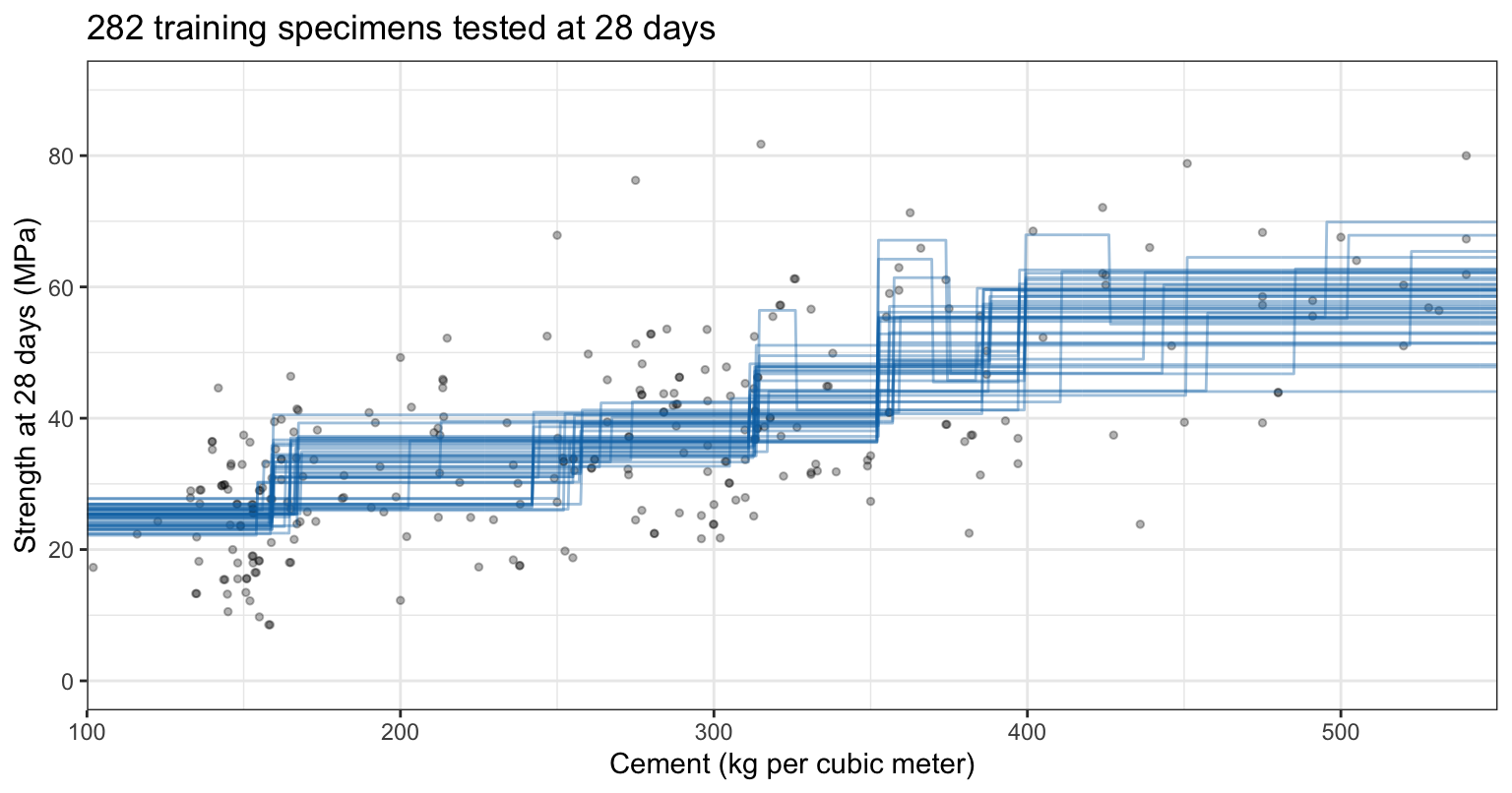
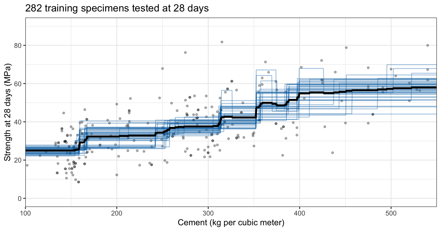
The 40 trees, from 20 halvings, put their steps in different places, and at a given cement content their predictions span up to 29.9 MPa. Over all 200 halvings, the most common first split, age < 21, is the first split of 74% of the 400 trees. The average of the 40 curves in the second tab is smoother than any one of them: it still steps, but in many small steps.
28.2.2 Averaging
At 300 kg of cement per cubic meter and 28 days, the 40 trees above predict between 32.7 and 42.5 MPa, with standard deviation 2.6; their average is 37.6. The variance of such an average follows from the variance and correlation of the predictions it averages.
Let \(\hat f_1(x), \ldots, \hat f_B(x)\) be \(B\) predictions at the same \(x\), each with variance \(\sigma^2\), and with correlation \(\rho\) between any two. The variance of their average is
\[ \begin{aligned} Var\left[\frac{1}{B}\sum_{b=1}^B \hat f_b(x)\right] &= \frac{1}{B^2}\left\{\sum_{b=1}^B Var\left[\hat f_b(x)\right] + \sum_{b \ne b'} Cov\left[\hat f_b(x), \hat f_{b'}(x)\right]\right\} \\ &= \frac{B\sigma^2 + B\left(B - 1\right)\rho\sigma^2}{B^2} = \rho\sigma^2 + \frac{1 - \rho}{B}\sigma^2, \end{aligned} \]
where
- \(B\) is the number of predictions averaged, indexed \(b = 1, \ldots, B\),
- \(\sigma^2\) is the variance of one prediction at \(x\) (in this lecture, not the error variance of a regression model), and
- \(\rho\) is the correlation between two of them.
With independent predictions, \(\rho = 0\), the variance falls like \(1/B\). With correlated ones it falls toward \(\rho\sigma^2\), the term that does not depend on \(B\).
28.2.3 Bootstrap samples
There is one training sample, not \(B\). Bagging, short for bootstrap aggregation, makes \(B\) training samples from it by resampling, as in the (optional) Bootstrap lecture: each bootstrap sample draws \(n\) observations from the \(n\) training observations at random with replacement. A given observation is missed by one draw with probability \(1 - 1/n\), and by all \(n\) independent draws with probability
\[\left(1 - \frac{1}{n}\right)^n \to e^{-1} \approx 0.368,\]
where \(n\) is the number of training observations and the limit, as \(n \to \infty\), is the case \(x = -1\) of \(\left(1 + x/n\right)^n \to e^x\); for \(n = 700\) the probability is 0.368. A bootstrap sample therefore contains about 63% of the distinct training observations, some of them more than once. The figure counts, for one bootstrap sample of the 700 training specimens, how many specimens appear 0, 1, 2, … times.
NoteCode
# One bootstrap sample of the training specimens, and how many times each
# specimen appears in it.
one_boot <- sample(n_train, replace = TRUE)
appearances <- tabulate(one_boot, nbins = n_train)
appear_counts <- as_tibble(table(times = appearances)) |>
  mutate(times = as.integer(times))
n_left_out <- sum(appearances == 0)

# Number of specimens: major lines every 50, minor lines midway.
count_axis <- scale_y_continuous(breaks = seq(0, 300, by = 50),
                                 minor_breaks = seq(25, 325, by = 50))
boot_plot <- ggplot(appear_counts, aes(x = factor(times), y = n)) +
  geom_col(fill = "grey70", color = "grey30") +
  count_axis +
  labs(x = "Times the specimen appears in the bootstrap sample",
       y = "Number of training specimens",
       title = paste("One bootstrap sample of", n_train,
                     "training specimens"))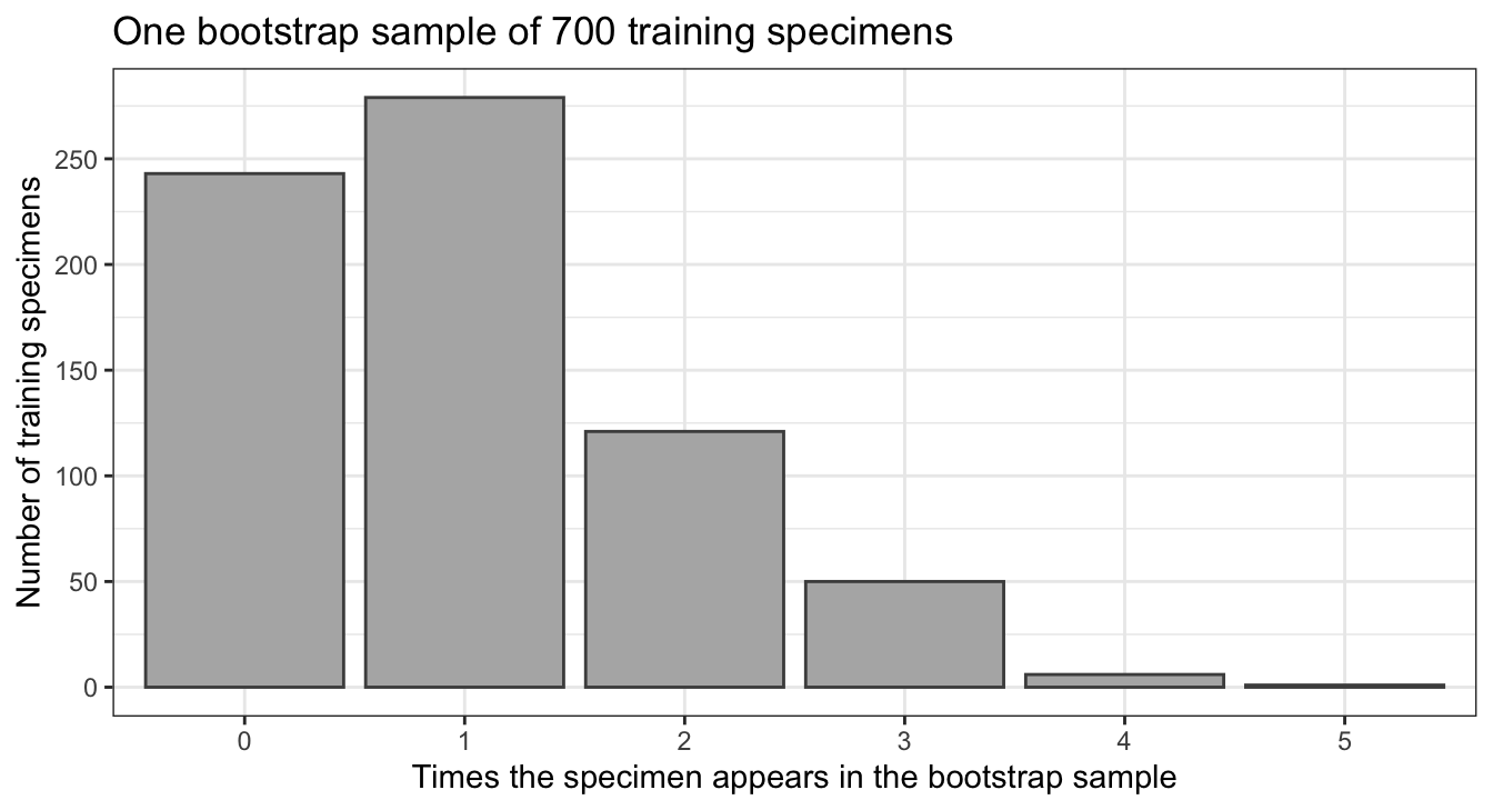
This bootstrap sample leaves out 243 of the 700 training specimens, 34.7%.
28.2.4 Bagged trees
Bagging fits a tree \(\hat f^{*b}\) to bootstrap sample \(b\), for \(b = 1, \ldots, B\), and predicts with their average,
\[\hat f_{\text{bag}}(x) = \frac{1}{B}\sum_{b=1}^B \hat f^{*b}(x),\]
where
- \(\hat f^{*b}(x)\) is the prediction at \(x\) of the tree fit to bootstrap sample \(b\), the star marking a quantity computed from a bootstrap sample, and
- \(\hat f_{\text{bag}}(x)\) is the bagged prediction.
The trees are grown full and not pruned: each has low bias and high variance, and the average removes much of the variance. For a class, each tree predicts a class, and the bagged prediction is the class most trees predict, a majority vote.
The chunk writes the bagging algorithm out with rpart(): \(B\) full trees on all 8 explanatory variables, each fit to its own bootstrap sample of the training specimens.
# Bagging from scratch: B full trees, each fit to a bootstrap sample.
B <- 300
grow <- rpart.control(cp = 0, minsplit = 2, minbucket = 1, xval = 0)
boots <- map(seq_len(B), \(b) sample(n_train, replace = TRUE))
trees <- map(boots, \(boot) {
  rpart(compressive_strength ~ ., data = train[boot, ], control = grow)
})
tree_pred <- sapply(trees, predict, newdata = test)
c(test_mse = mean((y_test - rowMeans(tree_pred))^2))
test_mse
26.76253 xval = 0 skips the cross-validation that rpart() would otherwise run in each fit; nothing is pruned. tree_pred holds one column of test predictions per tree, and the bagged prediction averages each row; here \(B = 300\).
NoteCode
# Test MSE of the average of the first k trees, for k = 1, ..., B.
bag_running <- t(apply(tree_pred, 1, cumsum)) /
  matrix(seq_len(B), nrow(test), B, byrow = TRUE)
bag_curve <- tibble(trees = seq_len(B),
                    test = colMeans((y_test - bag_running)^2))
bag_mse <- bag_curve$test[B]

# Test MSE of each single tree, and whether every one is above the full
# tree's.
single_mse <- colMeans((y_test - tree_pred)^2)
singles_above_full <- all(single_mse > monday_mse[["full"]])

# The number of trees from which a curve stays within a share `tol` of its
# last value, on either side.
settle_at <- function(curve, tol) {
  final <- tail(curve, 1)
  outside <- which(abs(curve - final) > tol * final)
  if (length(outside) == 0) 1 else max(outside) + 1
}
settle_share <- 0.05
settle_k <- settle_at(bag_curve$test, settle_share)
after_range <- range(bag_curve$test[seq(settle_k, B)])

# Number of trees: major lines every 50, minor lines midway.
trees_axis <- scale_x_continuous(breaks = seq(0, 500, by = 50),
                                 minor_breaks = seq(25, 525, by = 50))

# MSE: major lines every 20, minor lines midway; the curve at one tree is
# clipped.
mse_axis <- scale_y_continuous(breaks = seq(0, 100, by = 20),
                               minor_breaks = seq(10, 110, by = 20))
mse_ylim <- c(0, 80)
bag_plot <- ggplot(bag_curve, aes(x = trees, y = test)) +
  geom_hline(yintercept = monday_mse[["full"]], linetype = "dashed") +
  geom_line(color = okabe_ito[5]) +
  trees_axis +
  mse_axis +
  coord_cartesian(ylim = mse_ylim) +
  labs(x = "Number of bagged trees, k", y = "Test MSE (MPa squared)",
       title = paste(n_train, "training specimens, all",
                     ncol(specimens) - 1, "explanatory variables"),
       caption = "Dashed line: the full tree of the Decision Trees lecture.")
The figure plots the test MSE of the average of the first \(k\) trees, \(k = 1, \ldots, B\), against \(k\), with the full tree fit to all the training specimens as a dashed line.
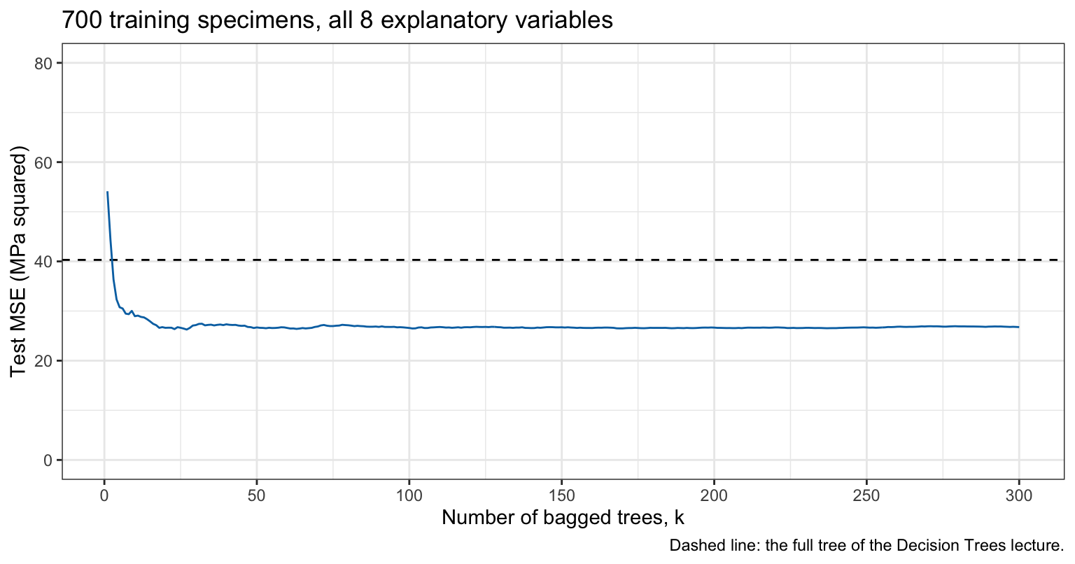
A single tree fit to a bootstrap sample has test MSE between 47.7 and 102.2; every one is above the full tree’s 40.3, and each sees only about 63% of the distinct specimens. Averaging brings the test MSE to 26.8 with 300 trees, and from \(k = 15\) on it stays within 5% of that value: what remains of the variance is the \(\rho\sigma^2\) term, which more trees do not reduce. The curve does not trend upward as trees are added: after \(k = 15\) it stays between 26.3 and 27.9, so adding trees does not overfit.
28.3 Out-of-bag error
28.3.1 Left-out specimens
Each bootstrap sample of the loop above leaves some training specimens out. The chunk records which, and counts them for the first five samples.
# Whether each training specimen is left out of each bootstrap sample, and
# how many are left out of the first five.
out_of_bag <- sapply(boots, \(boot) !(seq_len(n_train) %in% boot))
left_out <- colSums(out_of_bag)
setNames(left_out[1:5], paste("sample", 1:5))
sample 1 sample 2 sample 3 sample 4 sample 5
274 263 268 243 261 These samples leave out between 243 and 274 of the 700 training specimens, and the tree fit to each never saw them.
28.3.2 Out-of-bag prediction
The out-of-bag (OOB) prediction of a training specimen averages the predictions of only the trees whose bootstrap samples left it out, the trees that never saw it. The OOB MSE compares these predictions with the training responses:
\[\text{MSE}_{\text{OOB}} = \frac{1}{n}\sum_{i=1}^n \left(y_i - \hat f_{\text{OOB}}(x_i)\right)^2, \qquad \hat f_{\text{OOB}}(x_i) = \frac{1}{\left|\mathcal{O}_i\right|}\sum_{b \in \mathcal{O}_i} \hat f^{*b}(x_i),\]
where
- \(\mathcal{O}_i\) is the set of bootstrap samples that leave out training observation \(i\), and \(\left|\mathcal{O}_i\right|\) their number, and
- \(\hat f_{\text{OOB}}(x_i)\) is the OOB prediction of observation \(i\).
Every training observation is predicted by trees that did not use it, as a held-out fold is in cross-validation, but the OOB error comes from the bagged fit itself, with no refitting. Computed from the 300 trees of the loop:
# Each tree's predictions for the training specimens; each specimen's OOB
# prediction averages the trees that left it out.
train_pred <- sapply(trees, predict, newdata = train)
oob_pred <- rowSums(train_pred * out_of_bag) / rowSums(out_of_bag)
c(oob_mse = mean((y_train - oob_pred)^2))
oob_mse
27.03195
NoteCode
# Running sums over the first k trees of the out-of-bag predictions and of
# the number of out-of-bag trees, for each specimen.
oob_sum <- t(apply(train_pred * out_of_bag, 1, cumsum))
oob_count <- t(apply(out_of_bag, 1, cumsum))

# OOB MSE after k trees, once every specimen has an out-of-bag tree.
first_k <- which(colSums(oob_count == 0) == 0)[1]
oob_mse_k <- colMeans((y_train - oob_sum / oob_count)^2)
oob_mse_k[seq_len(first_k - 1)] <- NA
oob_mse <- oob_mse_k[B]

# Share of the trees each specimen is out of bag for.
oob_share <- rowMeans(out_of_bag)

# Share of the values of k, from first_k on, at which the OOB MSE is above
# the test MSE.
defined_k <- seq(first_k, B)
oob_above <- mean(oob_mse_k[defined_k] > bag_curve$test[defined_k])
oob_gap <- oob_mse_k[defined_k] - bag_curve$test[defined_k]

# Share of the training specimens whose mix, the seven ingredients, is the
# mix of another training specimen, and of the test specimens whose mix is
# that of some training specimen.
ingredients <- setdiff(names(train), c("age", "compressive_strength"))
train_mix_shared <- train |>
  add_count(across(all_of(ingredients)), name = "copies") |>
  summarise(share = mean(copies > 1)) |>
  pull(share)
train_mixes <- distinct(select(train, all_of(ingredients)))
test_mix_matches <- semi_join(test, train_mixes, by = ingredients)
test_mix_seen <- nrow(test_mix_matches) / nrow(test)

# Test and OOB MSE against the number of trees; the reference line is
# grey and dot-dashed, the OOB curve dashed.
curve_labels <- c("Test", "Out of bag")
oob_long <- bag_curve |>
  mutate(`Out of bag` = oob_mse_k) |>
  rename(Test = test) |>
  pivot_longer(-trees, names_to = "error", values_to = "mse") |>
  filter(!is.na(mse)) |>
  mutate(error = factor(error, levels = curve_labels))
oob_plot <- ggplot(oob_long, aes(x = trees, y = mse, color = error,
                                 linetype = error)) +
  geom_hline(yintercept = monday_mse[["full"]], linetype = "dotdash",
             color = "grey50") +
  geom_line() +
  scale_color_manual(values = okabe_ito[c(5, 4)]) +
  scale_linetype_manual(values = c("solid", "dashed")) +
  trees_axis +
  mse_axis +
  coord_cartesian(ylim = mse_ylim) +
  labs(x = "Number of bagged trees, k", y = "MSE (MPa squared)",
       color = NULL, linetype = NULL,
       title = paste(n_train, "training specimens, all",
                     ncol(specimens) - 1, "explanatory variables"),
       caption = "Dot-dashed line: the full tree's test MSE.") +
  theme(legend.position = "inside",
        legend.position.inside = c(0.99, 0.97),
        legend.justification = c(1, 1),
        legend.background = element_rect(color = "grey50"))
28.3.3 Out-of-bag and test error
Over the 300 trees, a training specimen is out of bag for between 30% and 45% of them, on average 36.9%. Every specimen has at least one out-of-bag tree among the first \(k\) from \(k = 15\) on. The figure plots the OOB MSE and the test MSE of the first \(k\) trees against \(k\).
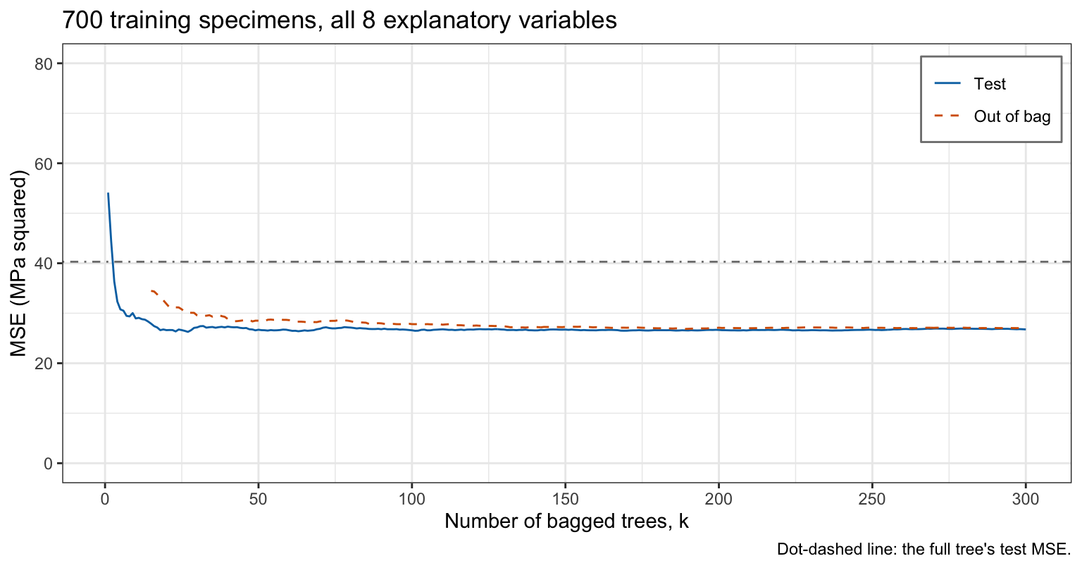
With 300 trees the OOB MSE is 27.0 and the test MSE 26.8. The OOB MSE is above the test MSE at every value of \(k\) from 15 to 300, by up to 6.9, most for few trees, where each specimen’s OOB prediction averages only a handful of trees. As with the test specimens in the Decision Trees lecture, the OOB error here measures predictions for mixes like those tested: 74% of the training specimens share their mix with another training specimen, often tested at another age, and 68% of the test specimens have a mix that some training specimen also has.
28.4 Random forests
28.4.1 Definition
A random forest combines three ingredients:
- bootstrap samples: each tree is fit to its own bootstrap sample of the training data,
- averaging: the forest predicts with the average of its trees’ predictions, or by majority vote for a class, and
- random variable inclusion: at each split, the tree chooses among only a random subset of the explanatory variables.
Bagged trees have the first two ingredients; the third is the one change a random forest makes to them.
28.4.2 Correlated trees
The figure counts the first split of each tree in two forests fit to all the training specimens with randomForest(): bagging, which may split on any of the 8 explanatory variables, and the random forest with randomForest()’s default \(m\), defined below.
NoteCode
# Bagging and a random forest with randomForest()'s default m, each with
# randomForest()'s default number of trees, on all the training specimens.
p <- ncol(specimens) - 1
bag_rf <- randomForest(compressive_strength ~ ., data = train, mtry = p)
default_rf <- randomForest(compressive_strength ~ ., data = train)
n_trees <- bag_rf$ntree

# The explanatory variable of the first split of each tree.
first_split <- function(forest) {
  map_chr(seq_len(forest$ntree), \(k) {
    tree <- getTree(forest, k, labelVar = TRUE)
    as.character(tree[1, "split var"])
  })
}
method_names <- c("Bagging", "Random forest")
roots <- bind_rows(tibble(method = method_names[1],
                          variable = first_split(bag_rf)),
                   tibble(method = method_names[2],
                          variable = first_split(default_rf)))
root_shares <- roots |>
  count(method, variable) |>
  mutate(share = n / sum(n), .by = method) |>
  complete(method, variable, fill = list(n = 0, share = 0)) |>
  mutate(method = factor(method, levels = method_names))
variable_order <- root_shares |>
  filter(method == "Bagging") |>
  arrange(share) |>
  pull(variable)
root_shares <- mutate(root_shares,
                      variable = factor(variable, levels = variable_order))
age_share <- root_shares |>
  filter(variable == "age") |>
  select(method, share) |>
  deframe()

# Share of trees: major lines every 20%, minor lines midway.
share_axis <- scale_x_continuous(breaks = seq(0, 1, by = 0.2),
                                 minor_breaks = seq(0.1, 0.9, by = 0.2),
                                 limits = c(0, 1),
                                 labels = scales::label_percent())
root_plot <- ggplot(filter(root_shares, share > 0),
                    aes(x = share, y = variable)) +
  geom_col(fill = "grey70", color = "grey30") +
  facet_wrap(~ method) +
  share_axis +
  scale_y_discrete(drop = FALSE) +
  labs(x = paste("Share of the", n_trees,
                 "trees whose first split uses the variable"),
       y = NULL, title = paste(n_train, "training specimens"))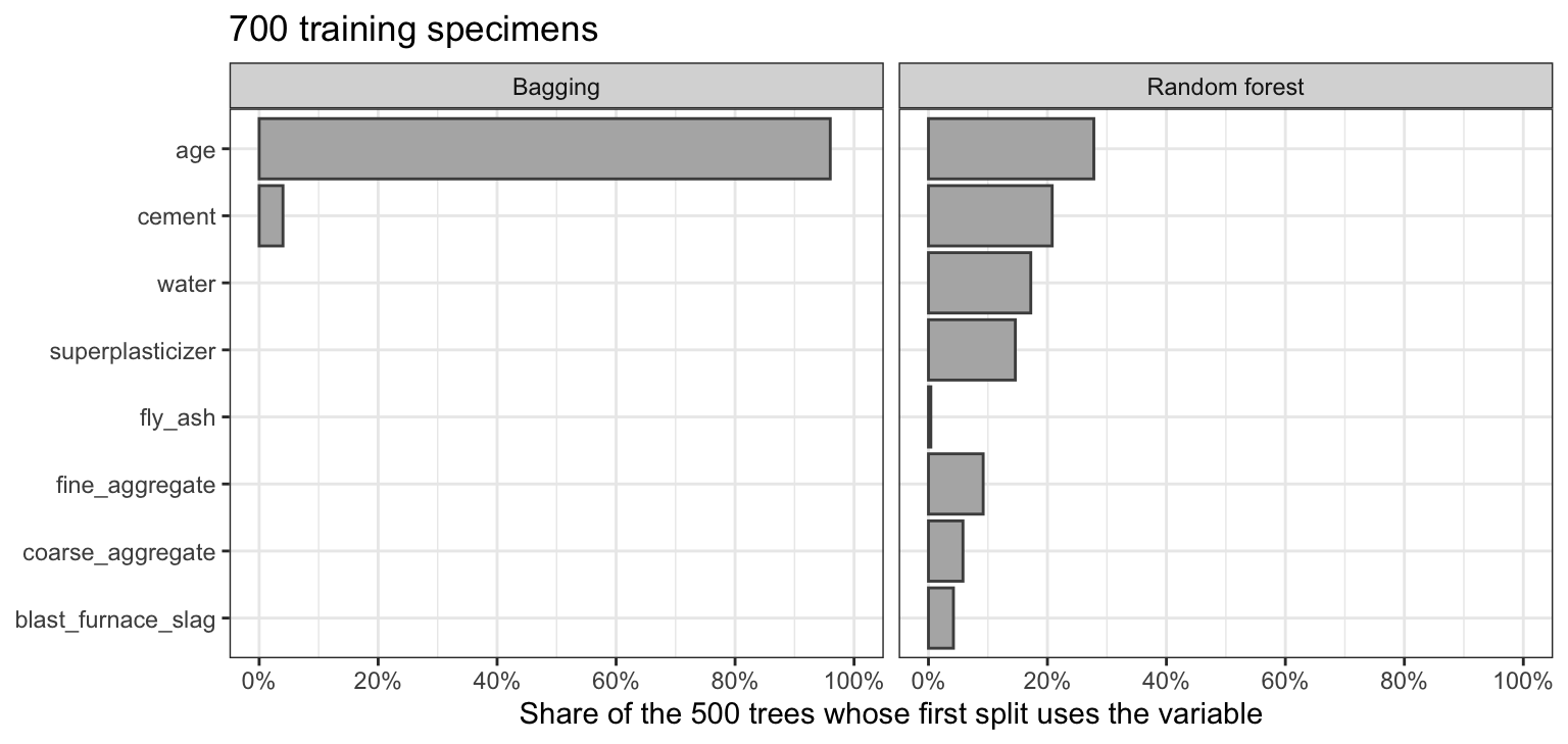
Each forest has 500 trees. In bagging, 96% of the trees split first on age; in the random forest, 28% do. Bagged trees are fit to overlapping samples of the same training data and nearly all begin with the same split.
28.4.3 Split restriction
NoteCode
# randomForest()'s default nodesize, read from the package, for a numeric
# response and for a class.
nodesize_default <- formals(randomForest:::randomForest.default)$nodesize
nodesize <- c(numeric = eval(nodesize_default, list(y = 0)),
              class = eval(nodesize_default, list(y = factor("a"))))

# Halvings and trees per forest for estimating the correlation below.
n_samples <- 100
n_small <- 100
The random subset of explanatory variables is the split restriction: at each split, the tree may use only \(m\) of the \(p\) explanatory variables, chosen at random anew for that split, where
- \(p\) is the number of explanatory variables, and
- \(m \le p\) is the number tried at each split.
\(m = p\) is bagging. A strong explanatory variable such as age is not available at many splits, including the first split of many trees, so the trees differ more, at the cost of some accuracy in each tree. randomForest() uses \(m = \lfloor p/3 \rfloor\) by default for a numeric response and \(m = \lfloor\sqrt{p}\rfloor\) for a class; for the 8 concrete explanatory variables the default is \(m = 2\). By its default nodesize, it does not split a node with 5 or fewer observations for a numeric response, or 1 or fewer for a class, so its regression trees are nearly, not exactly, full.
The correlation \(\rho\) and the variance \(\sigma^2\) can be estimated from the data, for trees fit to 350 specimens (a half), across random halvings of the training specimens. For each of 100 new halvings, a forest of 100 trees is fit to the first half, with \(m = p\) and with the default \(m\). At each test specimen, the variance of one tree’s prediction splits into two parts: the variance across halvings of the expected prediction of a forest, shared by all its trees, and the variance among the trees of one forest. The first part is the variance of the forests’ average predictions across halvings, less the variance among trees divided by 100, which an average of 100 trees still carries. These are values at one \(x\), the explanatory variables of one test specimen. The table averages them over the 305 test specimens: \(\hat\sigma^2\) is the average of the sum of the two parts, \(\hat\rho\hat\sigma^2\) is the average of the first part, and \(\hat\rho\) is their ratio.
NoteCode
# For one half of the training specimens and m, each test specimen's
# average prediction over the trees of a forest and the variance among
# the trees.
forest_moments <- function(rows, m) {
  forest <- randomForest(compressive_strength ~ ., data = train[rows, ],
                         mtry = m, ntree = n_small)
  individual <- predict(forest, test, predict.all = TRUE)$individual
  list(mean = rowMeans(individual),
       within = apply(individual, 1, var))
}

# Halvings; the forests of each method on the first half of each.
halves <- map(seq_len(n_samples), \(h) sample(n_train, n_train / 2))
m_values <- c(Bagging = p, `Random forest` = floor(p / 3))
correlations <- imap(m_values, \(m, method) {
  moments <- map(halves, \(rows) forest_moments(rows, m))
  means <- sapply(moments, \(x) x$mean)
  within <- rowMeans(sapply(moments, \(x) x$within))

  # The shared part: the variance of the forest averages across halvings,
  # less the Monte Carlo variance within / n_small of an average of n_small
  # trees; sigma^2 adds the variance among trees.
  shared <- apply(means, 1, var) - within / n_small
  sigma2_x <- shared + within
  tibble(method = method, m = m, sigma2 = mean(sigma2_x),
         shared = mean(shared), rho = mean(shared) / mean(sigma2_x))
}) |>
  list_rbind()
rho <- deframe(select(correlations, method, rho))
sigma2 <- deframe(select(correlations, method, sigma2))
shared <- deframe(select(correlations, method, shared))
correlation_table <- correlations |>
  transmute(method, m,
            sigma2 = fmt(sigma2, 0),
            rho = fmt(rho, 2),
            shared = fmt(shared, 1)) |>
  knitr::kable(col.names = c("Method", "$m$", "$\\hat\\sigma^2$",
                             "$\\hat\\rho$", "$\\hat\\rho\\hat\\sigma^2$"),
               align = "lrrrr")

# Mean test MSE of a single tree of each forest fit to all the training
# specimens.
single_tree_mse <- function(forest) {
  individual <- predict(forest, test, predict.all = TRUE)$individual
  mean(colMeans((y_test - individual)^2))
}
single_rf <- c(Bagging = single_tree_mse(bag_rf),
               `Random forest` = single_tree_mse(default_rf))

# The prose says the restriction lowers the correlation and raises the
# variance of one tree.
stopifnot(rho[["Random forest"]] < rho[["Bagging"]],
sigma2[["Random forest"]] > sigma2[["Bagging"]])| Method | \(m\) | \(\hat\sigma^2\) | \(\hat\rho\) | \(\hat\rho\hat\sigma^2\) |
|---|---|---|---|---|
| Bagging | 8 | 62 | 0.09 | 5.8 |
| Random forest | 2 | 105 | 0.04 | 4.4 |
With \(m = p\), \(\hat\rho = 0.09\); with \(m = 2\), \(\hat\rho = 0.04\). For these data the restriction lowers the correlation between trees and raises the variance of one tree, \(\hat\sigma^2\), from 62 to 105: it randomizes each tree’s splits, so the trees differ more, and each tree is a more variable predictor. The part that no number of trees removes, \(\hat\rho\hat\sigma^2\), is 5.8 for bagging and 4.4 for the random forest. These are variances for trees fit to 350 specimens (a half), across halvings of the 700 training specimens, which overlap, not across independent training samples; and they say nothing about bias.
The restriction also changes each tree. In the forests of 500 trees fit to all 700 training specimens, a single tree has mean test MSE 68.2 with \(m = p\) and 111.9 with \(m = 2\). Part of that loss is variance: \(\hat\sigma^2\) above is larger with the restriction. Averaging removes only the \(\left(1 - \rho\right)\sigma^2/B\) part of a tree’s variance.
28.4.4 Fitting
# A random forest with the default m and number of trees, and its test MSE.
rf_fit <- randomForest(compressive_strength ~ ., data = train,
                       importance = TRUE)
rf_fit
Call:
 randomForest(formula = compressive_strength ~ ., data = train,      importance = TRUE)
               Type of random forest: regression
                     Number of trees: 500
No. of variables tried at each split: 2

          Mean of squared residuals: 32.1988
% Var explained: 88.07c(test_mse = mean((y_test - predict(rf_fit, test))^2))test_mse
34.24721
NoteCode
# Test and OOB MSE of the forest, for the prose.
rf_mse <- mse(y_test, predict(rf_fit, test))
rf_oob <- tail(rf_fit$mse, 1)
The printout gives the number of trees, the \(m\) used (“variables tried at each split”), the OOB MSE (“mean of squared residuals”), 32.2, and “% Var explained”, one minus the OOB MSE divided by the variance (divisor \(n\)) of the training responses. The test MSE is 34.2.
28.4.5 Forest size
NoteCode
# Test MSE of the first k trees' average, for each k up to a forest's size.
running_test <- function(forest) {
  individual <- predict(forest, test, predict.all = TRUE)$individual
  ntree <- ncol(individual)
  running <- t(apply(individual, 1, cumsum)) /
    matrix(seq_len(ntree), nrow(test), ntree, byrow = TRUE)
  colMeans((y_test - running)^2)
}

# OOB and test MSE against the number of trees, for bagging and the
# random forest with the default m.
ntree_wide <- bind_rows(
  tibble(method = "Bagging", trees = seq_len(bag_rf$ntree),
         `Out of bag` = bag_rf$mse, Test = running_test(bag_rf)),
  tibble(method = "Random forest", trees = seq_len(rf_fit$ntree),
         `Out of bag` = rf_fit$mse, Test = running_test(rf_fit))
)
ntree_curves <- ntree_wide |>
  pivot_longer(c(`Out of bag`, Test), names_to = "error",
               values_to = "mse") |>
  mutate(method = factor(method, levels = method_names),
         error = factor(error, levels = c("Out of bag", "Test")))
ntree_end <- ntree_curves |>
  filter(trees == max(trees)) |>
  select(method, error, mse)
end_mse <- function(method_name, error_name) {
  ntree_end |>
    filter(method == method_name, error == error_name) |>
    pull(mse)
}

# The number of trees from which each curve stays within each share of its
# last value.
settle_tols <- c(0.05, 0.02)
settle_table <- ntree_curves |>
  summarise(within_5 = settle_at(mse, settle_tols[1]),
            within_2 = settle_at(mse, settle_tols[2]),
            .by = c(method, error)) |>
  arrange(method, error)
settle_display <- knitr::kable(
  settle_table,
  col.names = c("Method", "Error", paste("Within", pct(settle_tols, 0))),
  align = "llrr"
)
slowest <- slice_max(settle_table, within_5, n = 1, with_ties = FALSE)

# The prose says the variance floor fell while the test and OOB MSE rose.
stopifnot(shared[["Random forest"]] < shared[["Bagging"]],
          end_mse("Random forest", "Test") > end_mse("Bagging", "Test"),
          end_mse("Random forest", "Out of bag") >
            end_mse("Bagging", "Out of bag"))

# Values above the axis limit, clipped in the figure.
clipped <- any(ntree_curves$mse > mse_ylim[2])
clip_caption <- if (clipped) {
  paste("Values above", mse_ylim[2], "at the first trees are clipped.")
} else {
  NULL
}

# For each method, the number of trees from which the OOB MSE stays on the
# side of the test MSE it ends on.
oob_side <- ntree_wide |>
  mutate(above = `Out of bag` > Test) |>
  summarise(ends_above = last(above),
            from = max(which(above != last(above)), 0) + 1,
            .by = method)
side_text <- function(method_name) {
  row <- filter(oob_side, method == method_name)
  side <- if (row$ends_above) "above" else "below"
  paste0(side, " the test MSE from ", row$from, " trees on")
}
ntree_plot <- ggplot(ntree_curves, aes(x = trees, y = mse, color = method,
                                       linetype = method)) +
  geom_line() +
  facet_wrap(~ error) +
  scale_color_manual(values = okabe_ito[c(5, 4)]) +
  scale_x_continuous(breaks = seq(0, 500, by = 100),
                     minor_breaks = seq(50, 550, by = 100)) +
  mse_axis +
  coord_cartesian(ylim = mse_ylim) +
  labs(x = "Number of trees", y = "MSE (MPa squared)", color = NULL,
       linetype = NULL, title = paste(n_train, "training specimens"),
       caption = clip_caption) +
  theme(legend.position = "bottom")
The figure plots the OOB MSE and the test MSE of randomForest()’s bagging (\(m = p\)) and its random forest (default \(m\)) against the number of trees. randomForest() computes the OOB MSE after \(k\) trees from the specimens with at least one out-of-bag tree among them, so its curves start at one tree, where the loop’s OOB curve above started at \(k = 15\).
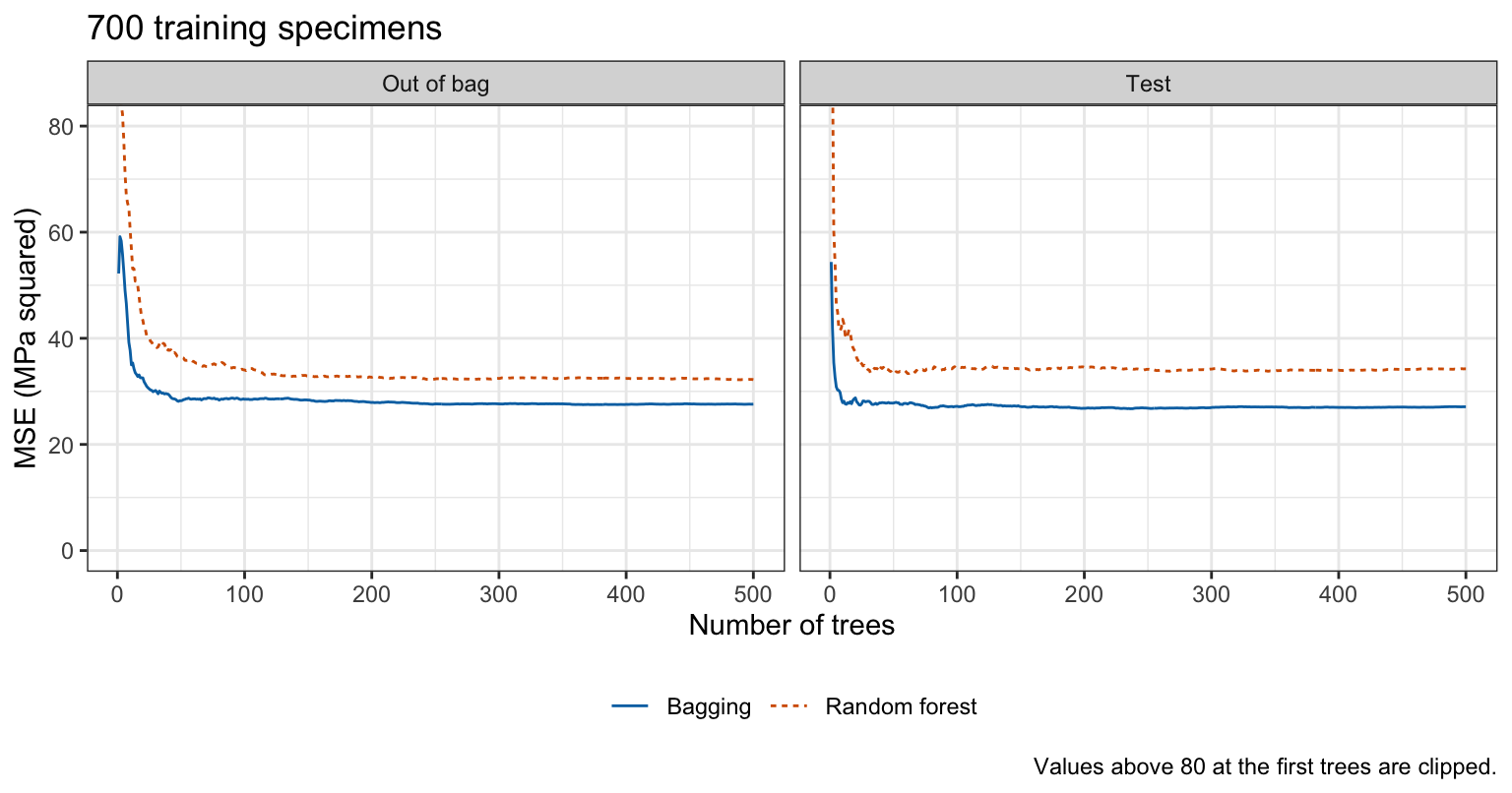
The table gives, for each curve, the number of trees from which it stays within 5% and within 2% of its value with 500 trees.
| Method | Error | Within 5% | Within 2% |
|---|---|---|---|
| Bagging | Out of bag | 42 | 186 |
| Bagging | Test | 21 | 67 |
| Random forest | Out of bag | 111 | 185 |
| Random forest | Test | 22 | 64 |
The slowest to settle within 5% is the out of bag curve of the random forest, at 111 trees, so 500 trees are enough here. With 500 trees, bagging has OOB MSE 27.6 and test MSE 27.1, and the random forest with \(m = 2\) has 32.2 and 34.2. The OOB MSE is above the test MSE from 2 trees on for bagging, and below the test MSE from 95 trees on for the random forest.
On these data the default \(m\) predicts worse than bagging. The Split restriction subsection shows why: the restriction lowered the variance that averaging cannot remove, \(\hat\rho\hat\sigma^2\), from 5.8 to 4.4, yet the forest’s test MSE rose from 27.1 to 34.2, and its OOB MSE moved the same way, from 27.6 to 32.2. The increase is mostly bias: with \(m = 2\) a tree often cannot split on the variables that matter most, and averaging does not remove that.
28.4.6 Choosing \(m\)
NoteCode
# A forest for each m from 1 to p, and its OOB and test MSE.
m_forests <- map(seq_len(p), \(m) {
  randomForest(compressive_strength ~ ., data = train, mtry = m)
})
m_curve <- tibble(m = seq_len(p),
                  `Out of bag` = map_dbl(m_forests, \(f) tail(f$mse, 1)),
                  Test = map_dbl(m_forests, \(f) {
                    mse(y_test, predict(f, test))
                  }))
m_best <- m_curve$m[which.min(m_curve$`Out of bag`)]
best_forest <- m_forests[[m_best]]

# The smallest m from which every m up to p has an OOB MSE within near_m
# of the smallest.
near_m <- 0.05
oob_near <- m_curve$`Out of bag` <= (1 + near_m) * min(m_curve$`Out of bag`)
m_flat <- max(which(!oob_near)) + 1
m_long <- m_curve |>
  pivot_longer(-m, names_to = "error", values_to = "mse") |>
  mutate(error = factor(error, levels = c("Out of bag", "Test")))
m_chosen <- filter(m_long, m == m_best, error == "Out of bag")
m_plot <- ggplot(m_long, aes(x = m, y = mse, color = error,
                             linetype = error, shape = error)) +
  geom_line() +
  geom_point(size = 2) +
  geom_point(data = m_chosen, size = 5, shape = 1, color = "black",
             show.legend = FALSE) +
  scale_color_manual(values = okabe_ito[c(4, 5)]) +
  scale_x_continuous(breaks = seq_len(p), minor_breaks = NULL) +
  scale_y_continuous(breaks = seq(0, 70, by = 10),
                     minor_breaks = seq(5, 75, by = 10),
                     limits = c(20, 70)) +
  labs(x = "Explanatory variables tried at each split, m",
       y = "MSE (MPa squared)", color = NULL, linetype = NULL,
       shape = NULL, title = paste(n_train, "training specimens"),
       caption = "Circle: the m with the smallest OOB MSE.") +
  theme(legend.position = "inside",
        legend.position.inside = c(0.99, 0.97),
        legend.justification = c(1, 1),
        legend.background = element_rect(color = "grey50"))
The OOB MSE chooses \(m\) without the test data. The figure plots the OOB and test MSE of a forest of 500 trees for each \(m\) from 1 to 8.
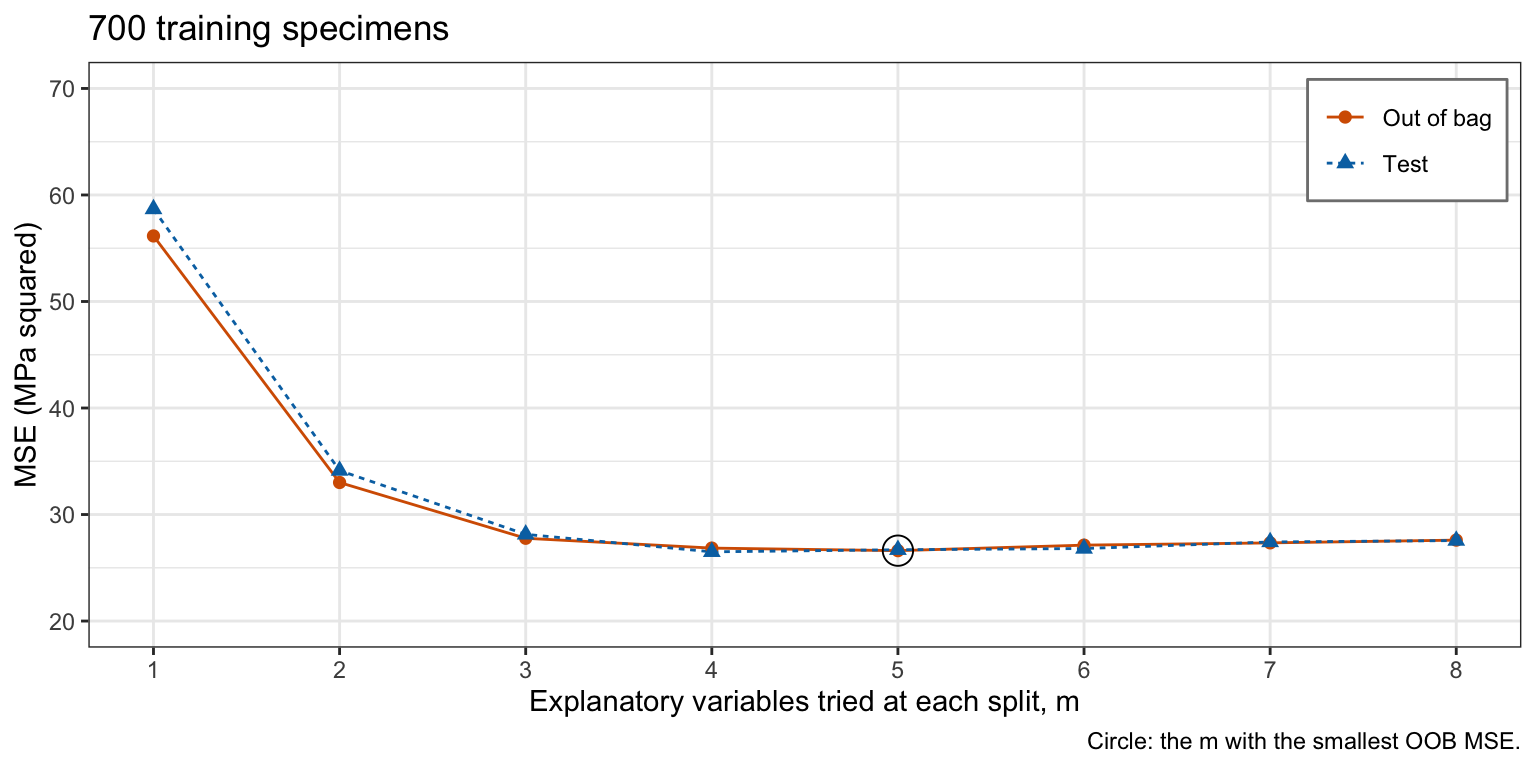
The OOB MSE is smallest at \(m = 5\), 26.6, and that forest’s test MSE is 26.7. With \(m = 1\) each split is on one variable chosen at random, and both errors are highest, 56.2 and 58.7. Every \(m\) from 3 to 8 has an OOB MSE within 5% of the smallest, so the choice among them matters little.
28.5 Variable importance
28.5.1 One tree
A single tree shows which explanatory variables it uses. The chunk refits the default tree of the Decision Trees lecture on all 8 explanatory variables and counts its splits on each.
# The default tree on all eight explanatory variables, and the number of
# its splits on each variable.
one_tree <- rpart(compressive_strength ~ ., data = train)
split_vars <- as.character(one_tree$frame$var)
table(split_vars[split_vars != "<leaf>"])
               age blast_furnace_slag             cement              water
                 5                  2                  4                  3
NoteCode
# The explanatory variables the tree splits on, and those it does not.
default_vars <- setdiff(unique(split_vars), "<leaf>")
unused_vars <- setdiff(names(train)[seq_len(p)], default_vars)
The tree never splits on fly_ash, superplasticizer, coarse_aggregate, and fine_aggregate. A forest of hundreds of trees has no single diagram to read, so it is summarized by two importance measures instead.
28.5.2 Two measures
Both measures are computed by randomForest() with importance = TRUE:
- Decrease in RSS (
IncNodePurity; for a class, the decrease in the Gini index): the total decrease in RSS from the splits on the variable in a tree, averaged over the trees. - Permutation importance (
%IncMSE; for a class,MeanDecreaseAccuracy): the increase in OOB MSE of each tree when the variable’s values are shuffled among that tree’s out-of-bag observations, with the tree not refit, averaged over the trees. Shuffling breaks the variable’s relation to the response. Withscale = FALSEthe increase is in the units of the MSE; by defaultimportance()divides it by its standard error.
# Both importance measures, the permutation increase in MPa squared.
importance(rf_fit, scale = FALSE)
%IncMSE IncNodePurity
cement 128.80824 38055.659
blast_furnace_slag 40.40708 10765.080
fly_ash 30.74548 9337.777
water 95.72834 22962.469
superplasticizer 68.02636 15163.163
coarse_aggregate 32.06984 13284.344
fine_aggregate 44.18691 14802.340
age 164.19623 54983.954
NoteCode
# Both measures, each variable ordered by the permutation measure.
importance_values <- importance(rf_fit, scale = FALSE) |>
  as_tibble(rownames = "variable") |>
  rename(permutation = `%IncMSE`, rss = IncNodePurity) |>
  arrange(permutation) |>
  mutate(variable = factor(variable, levels = variable))
permutation_rank <- rev(levels(importance_values$variable))
rss_rank <- importance_values |>
  arrange(desc(rss)) |>
  pull(variable) |>
  as.character()

# One dot chart per measure, side by side.
dot_chart <- function(column, label, breaks, minor, labels = waiver()) {
  ggplot(importance_values, aes(x = .data[[column]], y = variable)) +
    geom_segment(aes(x = 0, xend = .data[[column]], yend = variable),
                 color = "grey60") +
    geom_point(size = 2.5) +
    scale_x_continuous(breaks = breaks, minor_breaks = minor,
                       limits = range(breaks), labels = labels) +
    labs(x = label, y = NULL)
}
rss_step <- 10000
rss_top <- ceiling(max(importance_values$rss) / rss_step) * rss_step
perm_step <- 50
perm_top <- ceiling(max(importance_values$permutation) / perm_step) *
  perm_step
permutation_plot <- dot_chart("permutation",
                              "Increase in OOB MSE (MPa squared)",
                              seq(0, perm_top, by = perm_step),
                              seq(perm_step / 2, perm_top, by = perm_step))
rss_plot <- dot_chart("rss", "Decrease in RSS (MPa squared)",
                      seq(0, rss_top, by = rss_step),
                      seq(rss_step / 2, rss_top, by = rss_step),
                      labels = scales::label_comma()) +
  theme(axis.text.y = element_blank())

# Whether every variable has a positive decrease in RSS in the forest.
all_used <- all(importance_values$rss > 0)

# Whether the two measures order the variables the same way, and whether
# they put the same variable first.
same_order <- identical(permutation_rank, rss_rank)
same_first <- permutation_rank[1] == rss_rank[1]
importance_plot <- patchwork::wrap_plots(permutation_plot, rss_plot) +
  patchwork::plot_annotation(
    title = paste("Random forest, m =", rf_fit$mtry, "of", p)
  )
The figure plots both measures for the random forest of the Fitting subsection of Random forests, the variables in the order of the permutation measure.
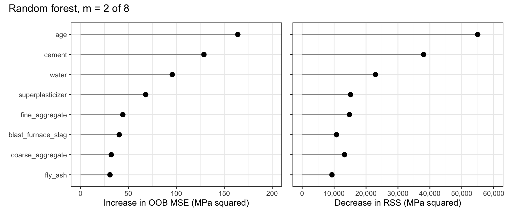
By permutation importance the order is age, cement, water, superplasticizer, fine_aggregate, blast_furnace_slag, coarse_aggregate, and fly_ash; by the decrease in RSS it is age, cement, water, superplasticizer, fine_aggregate, coarse_aggregate, blast_furnace_slag, and fly_ash. Both put age first. In the forest every variable has a positive decrease in RSS, so every one is split on somewhere, including those the single tree never used: with \(m = 2\), a given variable is among those tried at a split with probability \(m/p = 0.25\), so the strongest are often unavailable.
28.5.3 Interpretation
Importance ranks the variables; it gives no direction and no effect size. A large importance for water says that the forest relies on it, through large decreases in RSS or through worse out-of-bag predictions when its values are shuffled, not whether concrete gets stronger or weaker as water increases, with the others fixed, or by how much. The two measures order the variables differently here: they measure different things, the fit to the training data within each tree and the loss of out-of-bag accuracy when the variable is shuffled.
28.6 Classification forests
28.6.1 Penguin species
The penguins are those of the Decision Trees lecture, 240 training penguins and 4 body measurements. The figure plots bill length against flipper length for the training penguins.
NoteCode
# Species colors and shapes, as in the Decision Trees lecture.
species_levels <- levels(penguins$species)
species_colors <- setNames(okabe_ito[c(1, 5, 3)], species_levels)
species_shapes <- setNames(c(16, 17, 15), species_levels)
penguin_plot <- ggplot(penguin_train,
                       aes(x = flipper_length_mm, y = bill_length_mm,
                           color = species, shape = species)) +
  geom_point(size = 2) +
  scale_color_manual(values = species_colors) +
  scale_shape_manual(values = species_shapes) +
  scale_x_continuous(breaks = seq(170, 230, by = 10),
                     minor_breaks = seq(175, 235, by = 10),
                     limits = c(170, 235), expand = expansion(0)) +
  scale_y_continuous(breaks = seq(30, 60, by = 5),
                     minor_breaks = seq(32.5, 57.5, by = 5),
                     limits = c(30, 60), expand = expansion(0)) +
  labs(x = "Flipper length (mm)", y = "Bill length (mm)", color = NULL,
       shape = NULL,
       title = paste(nrow(penguin_train), "training penguins")) +
  theme(legend.position = "bottom")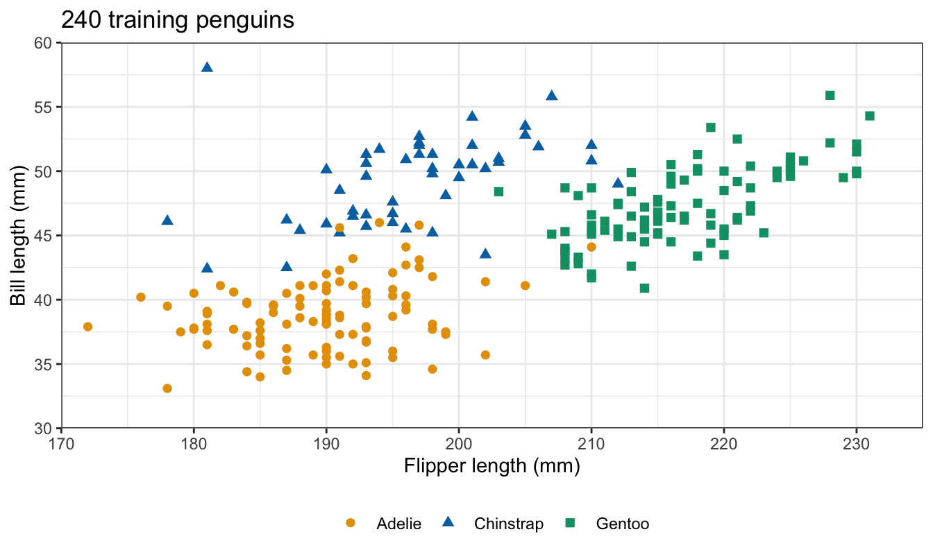
A random forest for a class works the same way as for a numeric response, with the Gini index for the splits, \(m = \lfloor\sqrt{p}\rfloor\) by default, and a majority vote over the trees.
28.6.2 Penguin forest
# A classification forest on the four measurements.
penguin_rf <- randomForest(species ~ bill_length_mm + bill_depth_mm +
                             flipper_length_mm + body_mass_g,
                           data = penguin_train, importance = TRUE)
penguin_rf
Call:
 randomForest(formula = species ~ bill_length_mm + bill_depth_mm +      flipper_length_mm + body_mass_g, data = penguin_train, importance = TRUE)
               Type of random forest: classification
                     Number of trees: 500
No. of variables tried at each split: 2

        OOB estimate of  error rate: 3.33%
Confusion matrix:
          Adelie Chinstrap Gentoo class.error
Adelie        99         2      1  0.02941176
Chinstrap      4        44      0  0.08333333
Gentoo         0         1     89  0.01111111
The printout gives the OOB error rate and the OOB confusion matrix, each training penguin classified by the trees for which it was out of bag.
# Predicted species of the test penguins, against their species.
penguin_pred <- predict(penguin_rf, penguin_test)
table(Predicted = penguin_pred, Observed = penguin_test$species)
Observed
Predicted Adelie Chinstrap Gentoo
Adelie 49 1 0
Chinstrap 0 19 0
Gentoo 0 0 33c(accuracy = mean(penguin_pred == penguin_test$species)) accuracy
0.9901961
NoteCode
# OOB error, test accuracy, and the test penguins each model gets right.
penguin_oob <- tail(penguin_rf$err.rate[, "OOB"], 1)
rf_accuracy <- accuracy_of(penguin_pred)
n_test_penguins <- nrow(penguin_test)
right <- round(c(tree_accuracy, forest = rf_accuracy) * n_test_penguins)

# Importance of the four measurements: decrease in Gini index, and the
# permutation decrease in OOB accuracy.
penguin_importance <- importance(penguin_rf, scale = FALSE)
gini_rank <- names(sort(penguin_importance[, "MeanDecreaseGini"],
                        decreasing = TRUE))
accuracy_rank <- names(sort(penguin_importance[, "MeanDecreaseAccuracy"],
                            decreasing = TRUE))

# OOB error and test accuracy for each m from 1 to 4.
penguin_m <- map(seq_along(measurements), \(m) {
  forest <- randomForest(penguin_formula, data = penguin_train, mtry = m)
  tibble(m = m,
         oob = tail(forest$err.rate[, "OOB"], 1),
         test = accuracy_of(predict(forest, penguin_test)))
}) |>
  list_rbind()

# The largest differences among the m, in penguins.
oob_spread <- round(diff(range(penguin_m$oob)) * nrow(penguin_train))
test_spread <- round(diff(range(penguin_m$test)) * n_test_penguins)
penguin_m_table <- penguin_m |>
  mutate(oob = pct(oob), test = pct(test)) |>
  knitr::kable(col.names = c("$m$", "OOB error rate", "Test accuracy"),
               align = "rrr")
The forest’s OOB error rate is 3.3%, and it classifies 99.0% of the 102 test penguins correctly, 101 of them. The default tree of the Decision Trees lecture classified 97 correctly (95.1%) and the pruned tree 98 (96.1%): the forest gets 3 more test penguins right than the better tree. On 102 test penguins a difference of a few penguins is small evidence. The decrease in Gini index and the permutation decrease in accuracy both rank the measurements bill_length_mm, flipper_length_mm, bill_depth_mm, and body_mass_g.
28.6.3 Choosing \(m\) for penguins
The table gives the OOB error rate and test accuracy of a forest for each \(m\) from 1 to 4.
| \(m\) | OOB error rate | Test accuracy |
|---|---|---|
| 1 | 2.9% | 99.0% |
| 2 | 3.3% | 99.0% |
| 3 | 3.3% | 99.0% |
| 4 | 3.8% | 98.0% |
The OOB error rates differ by at most 2 of the 240 training penguins, and the test accuracies by at most 1 of the 102 test penguins, so no choice of \(m\) stands out.
28.7 Comparison
28.7.1 Test error
NoteCode
# Test MSE on the concrete specimens, and test accuracy on the penguins.
concrete_rows <- tribble(
  ~Method, ~value,
  "Least squares, main effects", monday_mse[["ls"]],
  "Least squares, main effects, log(age)", monday_mse[["log_ls"]],
  "Default tree", monday_mse[["default"]],
  "Pruned tree", monday_mse[["pruned"]],
  "Full tree", monday_mse[["full"]],
  "Bagging, rpart() loop", bag_mse,
  "Bagging, randomForest()", end_mse("Bagging", "Test"),
  paste0("Random forest, m = ", floor(p / 3)), rf_mse,
  paste0("Random forest, m = ", m_best), m_curve$Test[m_best]
) |>
  mutate(value = fmt(value, 1))
concrete_table <- knitr::kable(concrete_rows,
                               col.names = c("Method", "Test MSE"),
                               align = "lr")
penguin_rows <- tibble(
  Method = c("Default tree", "Pruned tree",
             paste0("Random forest, m = ", penguin_rf$mtry)),
  accuracy = pct(c(tree_accuracy, rf_accuracy)),
  right = paste(right, "of", n_test_penguins)
)
penguin_table <- knitr::kable(penguin_rows,
                              col.names = c("Method", "Test accuracy",
                                            "Correct"),
                              align = "lrr")

# Whether every average of trees beats every single tree and least squares
# with main effects.
ensemble_mse <- c(bag_mse, end_mse("Bagging", "Test"), rf_mse,
                  m_curve$Test[m_best])
single_mse_min <- min(monday_mse[c("ls", "default", "pruned", "full")])
all_beat <- max(ensemble_mse) < single_mse_min
best_ensemble <- min(ensemble_mse)

# Bagging's Monte Carlo spread: the test MSE of the loop's first and
# second halves of trees.
half_B <- B / 2
half_mse <- c(mse(y_test, rowMeans(tree_pred[, seq_len(half_B)])),
              mse(y_test, rowMeans(tree_pred[, -seq_len(half_B)])))
The tables give the test MSE on the concrete test specimens and the test accuracy on the test penguins. Both least squares fits have main effects only: each explanatory variable enters linearly, with no interactions or polynomial terms, and the second replaces age by \(\log(\texttt{age})\). Least squares with quadratic terms or interactions is not in the table.
| Method | Test MSE |
|---|---|
| Least squares, main effects | 106.4 |
| Least squares, main effects, log(age) | 48.5 |
| Default tree | 86.8 |
| Pruned tree | 42.2 |
| Full tree | 40.3 |
| Bagging, rpart() loop | 26.8 |
| Bagging, randomForest() | 27.1 |
| Random forest, m = 2 | 34.2 |
| Random forest, m = 5 | 26.7 |
| Method | Test accuracy | Correct |
|---|---|---|
| Default tree | 95.1% | 97 of 102 |
| Pruned tree | 96.1% | 98 of 102 |
| Random forest, m = 2 | 99.0% | 101 of 102 |
On concrete, every average of trees beats every single tree and least squares with main effects; the best average has test MSE 26.7, against 40.3 for the best single tree and 48.5 for least squares with main effects and \(\log(\texttt{age})\), a feature built for the curvature in age. The two bagging fits, 26.8 and 27.1, differ in their bootstrap samples and in node size (full trees against randomForest()’s nodesize = 5); the first and second 150 trees of the loop alone give 26.7 and 27.1, a spread at least as large.
28.7.2 Extrapolation
NoteCode
# A grid of cement at 28 days, the other ingredients at their medians.
medians <- summarise(train, across(all_of(ingredients), median))
wide_grid <- tibble(cement = seq(100, 800, by = 2)) |>
  bind_cols(select(medians, -cement)) |>
  mutate(age = 28)
max_cement <- max(train$cement)
extrapolation_curves <- bind_rows(
  mutate(wide_grid, strength = predict(best_forest, wide_grid),
         fit = paste0("Random forest, m = ", m_best)),
  mutate(wide_grid, strength = predict(log_ls, wide_grid),
         fit = "Least squares with log(age)")
)

# Forest prediction at the largest training cement and at the end of the
# grid.
forest_at <- function(c) {
  prediction <- predict(best_forest, mutate(medians, cement = c, age = 28))
  unname(prediction)
}
forest_flat <- c(at_max = forest_at(max_cement), at_end = forest_at(800))
extrapolation_plot <- ggplot(extrapolation_curves,
                             aes(x = cement, y = strength, color = fit,
                                 linetype = fit)) +
  geom_vline(xintercept = max_cement, linetype = "dashed",
             color = "grey40") +
  geom_line(linewidth = 0.9) +
  scale_color_manual(values = okabe_ito[c(4, 5)]) +
  scale_x_continuous(breaks = seq(100, 800, by = 100),
                     minor_breaks = seq(150, 750, by = 100)) +
  scale_y_continuous(breaks = seq(0, 100, by = 20),
                     minor_breaks = seq(10, 90, by = 20),
                     limits = c(0, 100)) +
  labs(x = "Cement (kg per cubic meter)",
       y = "Predicted strength at 28 days (MPa)", color = NULL,
       linetype = NULL,
       title = "Other ingredients at their training medians",
       caption = "Dashed line: the largest cement among training specimens.") +
  theme(legend.position = "inside",
        legend.position.inside = c(0.01, 0.97),
        legend.justification = c(0, 1),
        legend.background = element_rect(color = "grey50"))
The figure plots the predicted strength at 28 days against cement, from 100 to 800 kg per cubic meter, with the other 6 ingredients at their training medians, for the random forest with the OOB-chosen \(m\) and for least squares with \(\log(\texttt{age})\); the dashed line is the largest cement content among the training specimens.
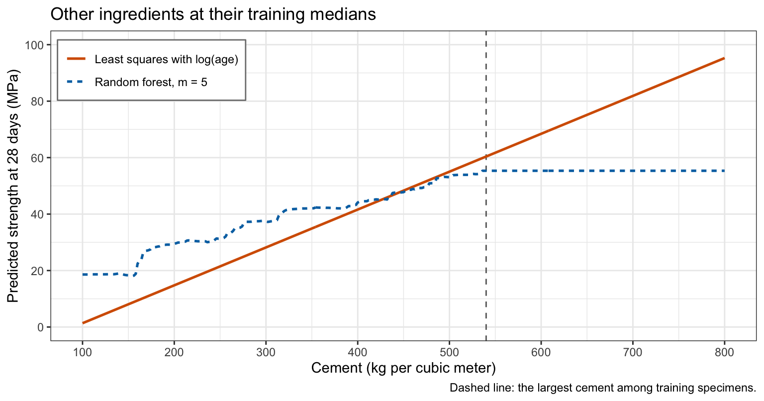
The forest predicts 55.3 MPa at the largest training cement content, 540, and 55.3 MPa at 800; least squares continues its line. Each tree predicts a constant beyond the largest value of an explanatory variable in its training sample, so a forest’s average does too. No data check either fit past 540.
28.7.3 Interpretability and cost
A forest gives up the single tree’s interpretability, leaving only importance rankings. It fits hundreds of trees instead of one, each of which must be stored and evaluated to predict. Its predictions are still made of steps.
NoteBeyond this course
- Extremely randomized trees. Choosing the cut point of each split at random as well as the variables decorrelates the trees further.
- Conditional forests. Forests of the conditional inference trees of the Decision Trees lecture’s pointer (
partykit::cforest()) avoid the bias of importance toward variables with many cut points. - Quantile regression forests. Keeping the training responses in each leaf, rather than their mean, estimates the conditional distribution of the response, and so prediction intervals.
- Proximity. The share of trees in which two observations land in the same leaf measures how similar they are;
randomForest(proximity = TRUE)returns it, for clustering or for finding outliers. - Faster implementations. The
rangerpackage fits the same forests much faster on large data.
28.8 Conclusion
Averaging \(B\) predictions with variance \(\sigma^2\) and pairwise correlation \(\rho\) gives variance \(\rho\sigma^2 + \left(1 - \rho\right)\sigma^2/B\): averaging removes the second term and leaves the first. Bagging applies this to trees. It fits one full, unpruned tree to each of \(B\) bootstrap samples of the training data, each sample leaving out about \(1/e\) of the observations, and averages their predictions, or takes a majority vote for a class. Adding trees does not overfit; the error levels off once the second term is small.
The observations a bootstrap sample leaves out give each training observation an out-of-bag prediction from the trees that never saw it, so the out-of-bag error estimates the test error from the fit itself, the role cross-validation played for single models.
Bagged trees tend to make the same strong splits, so they are correlated and the \(\rho\sigma^2\) term remains. A random forest lets each split choose among only \(m\) randomly chosen explanatory variables, which decorrelates the trees at some cost in the accuracy of each; \(m = p\) is bagging, and \(m\) is chosen by the out-of-bag error. A forest is read through variable importance, the decrease in RSS or Gini index from each variable’s splits, or the increase in out-of-bag error when the variable is shuffled, which ranks the variables but gives no direction or effect size. Forests usually predict better than one tree, at the cost of interpretability, and like a tree they cannot extrapolate.
The next lecture covers boosting, which also combines many trees, but builds them one after another, each fit to the residuals of the trees before it, instead of in parallel on bootstrap samples.