18 Cross-Validation in Practice

Learning objectives

After this lecture you should be able to

explain why the smallest cross-validation estimate among many candidate models tends to underestimate the test error of the model it selects, and predict how that optimism changes with the number of candidates, the noise in their estimates, and the correlation between them,
describe a workflow that keeps test data out of every choice: split off the test data first; choose by cross-validation on the training data only, with every data-dependent step of fitting (here, standardization) repeated inside each fold and the features and tuning parameters chosen by comparing the cross-validation estimates; refit the chosen model to all the training data; and evaluate it once on the test data,
classify the data used at each step of an analysis as training, validation, or test data, and identify which choices used which, and
explain why test data that have been used to choose among models no longer give an honest estimate of the chosen model’s test error.

18.1 Ames home sales

Question. How accurately can the sale price of a home in Ames, Iowa, be predicted from its size, age, and location, and which model should make the predictions?

Data. modeldata::ames records 2,930 home sales in Ames from 2006 to 2010. The response is the sale price, Sale_Price, analyzed as $\log_{10}$ of the price in dollars: prices are right-skewed, and an error on the $\log_{10}$ scale is a relative error, so a $20,000 miss counts more on a $100,000 home than on a $400,000 one. The explanatory variables are, in this order, above-ground living area (Gr_Liv_Area), year built (Year_Built), basement area (Total_Bsmt_SF), garage area (Garage_Area), and the home’s Longitude and Latitude. The tabs plot the sale price against living area, against each of the six explanatory variables, and on a map.

Code

homes <- modeldata::ames |>
  mutate(log_price = log10(Sale_Price))
n_homes <- nrow(homes)

explanatory <- c(Gr_Liv_Area = "Living area (sq ft)", Year_Built = "Year built",
                 Total_Bsmt_SF = "Basement area (sq ft)",
                 Garage_Area = "Garage area (sq ft)",
                 Longitude = "Longitude", Latitude = "Latitude")
vars <- names(explanatory)
big_area <- 4000
n_big <- sum(homes$Gr_Liv_Area > big_area)

price_axis <- scale_y_log10(breaks = c(25, 50, 100, 200, 400, 800) * 1000,
                            labels = dollars)
living_plot <- ggplot(homes, aes(x = Gr_Liv_Area, y = Sale_Price)) +
  geom_point(alpha = 0.25, size = 0.8) +
  price_axis +
  labs(x = "Living area (sq ft)", y = "Sale price (log scale)",
       title = "modeldata::ames")
six_plot <- homes |>
  pivot_longer(all_of(vars), names_to = "variable") |>
  mutate(variable = factor(explanatory[variable], levels = explanatory)) |>
  ggplot(aes(x = value, y = Sale_Price)) +
  geom_point(alpha = 0.15, size = 0.4) +
  facet_wrap(~ variable, scales = "free_x") +
  price_axis +
  labs(x = NULL, y = "Sale price (log scale)", title = "modeldata::ames")
map_plot <- ggplot(arrange(homes, Sale_Price),
                   aes(x = Longitude, y = Latitude, color = Sale_Price)) +
  geom_point(size = 0.7) +
  scale_color_viridis_c(trans = "log10", labels = dollars,
                        breaks = c(50, 100, 200, 400) * 1000) +
  coord_quickmap() +
  labs(color = "Sale price", title = "modeldata::ames")

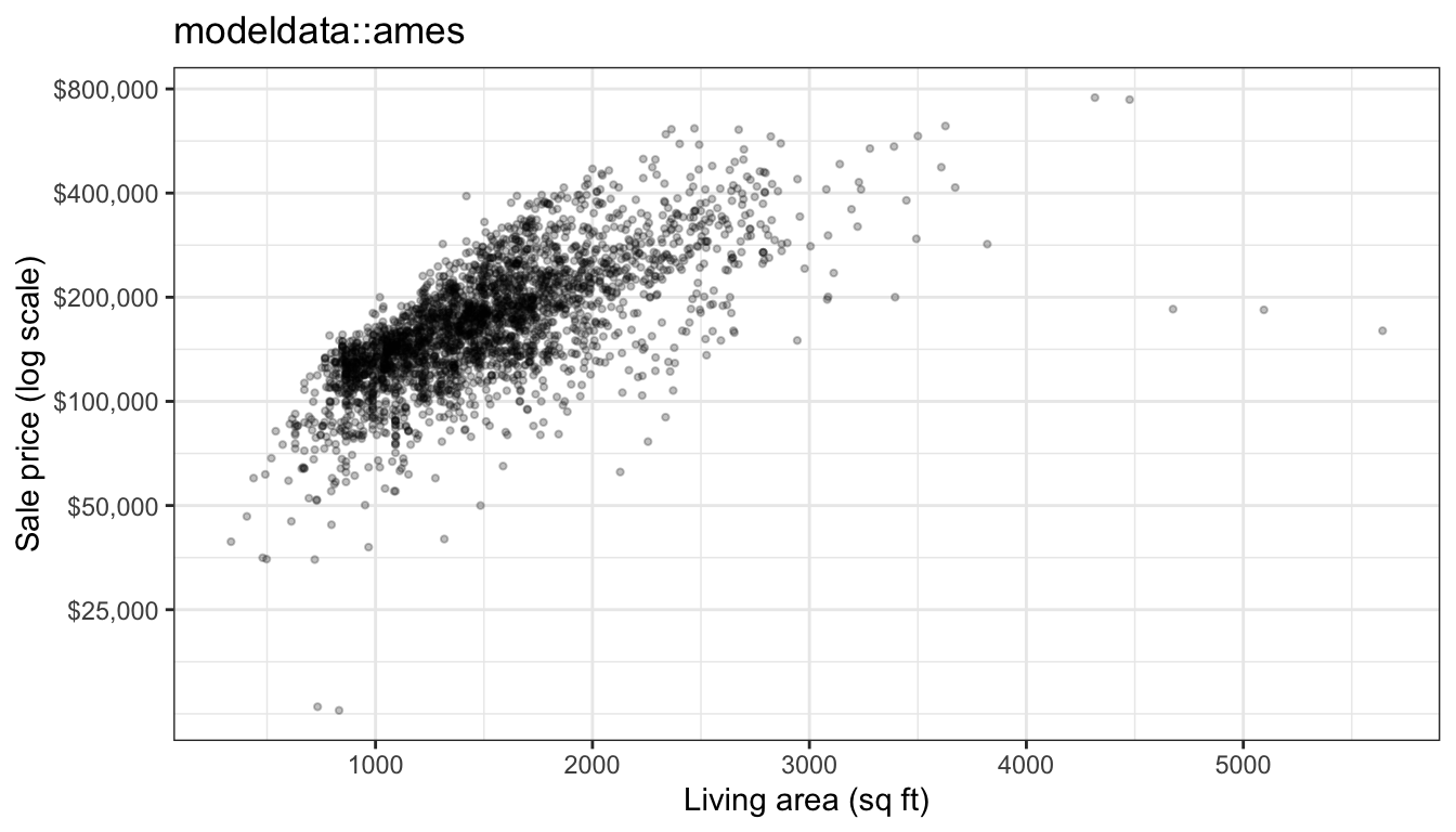
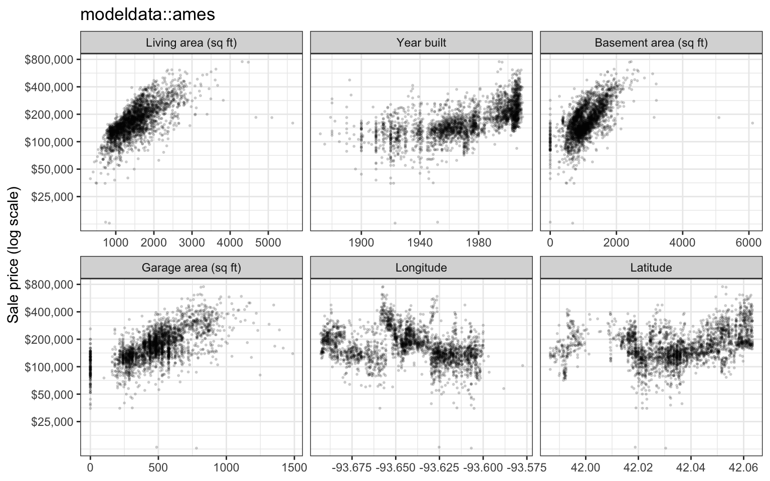
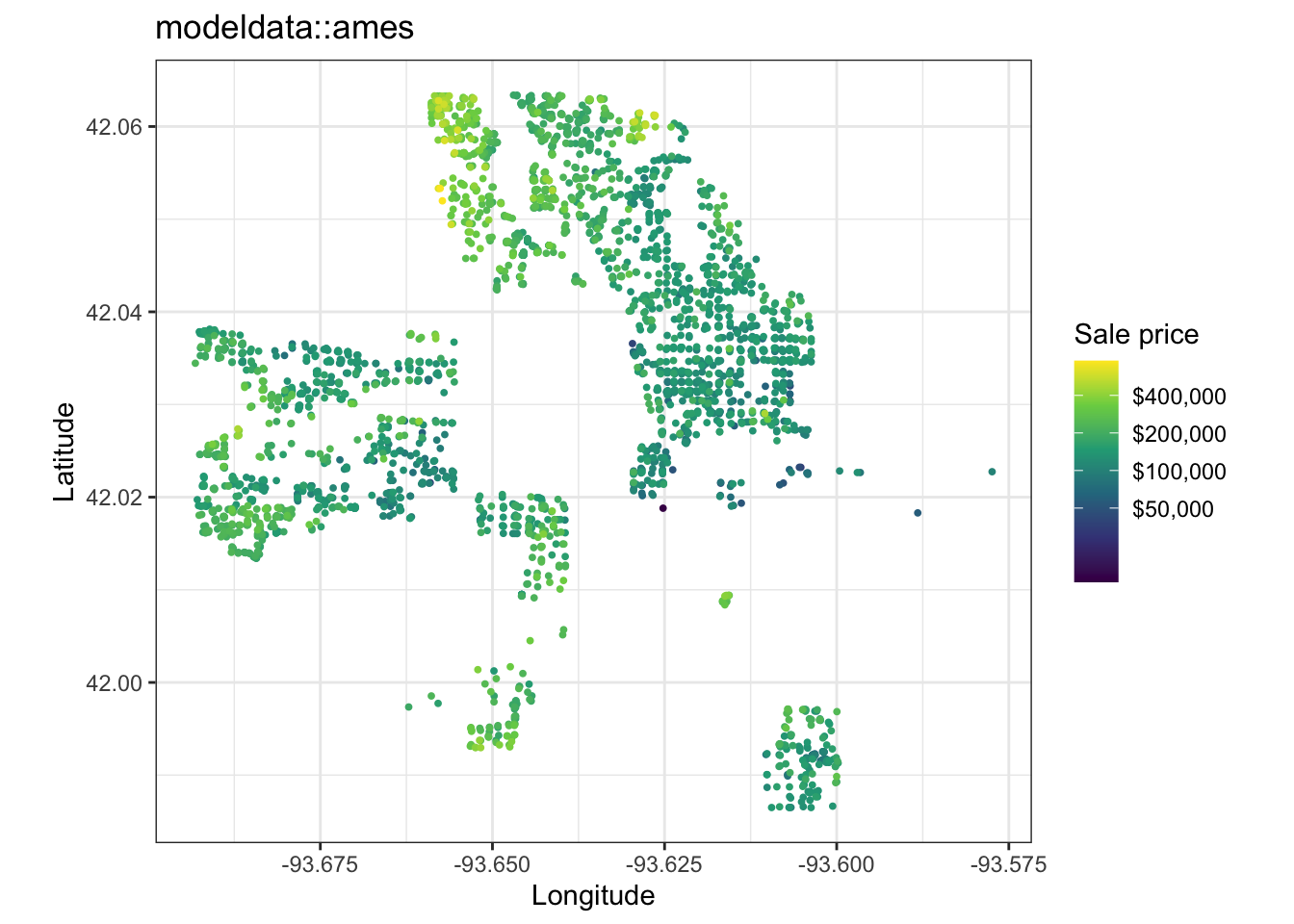
On the log scale, price rises roughly linearly with living area, with a few exceptions: 5 homes have more than 4,000 square feet, and some of them sold for far less than the trend. Newer homes, and homes with larger basements and garages, also sell for more; the vertical stripe at zero basement area is the homes without a basement. On the map, the most expensive homes are in the north of the city and the least expensive in its center and east, so nearby homes sell for similar prices.

18.2 Candidate models

m <- 200
one_id <- sample(n_homes, m)
show_K <- c(1, 15, 40)

A training sample of 200 homes, drawn at random from the 2,930, will be used to choose a model. The first tab shows it (black) against the other 2,730 homes (grey). The other tabs add KNN fits that use living area only, with $K$ = 1, 15, and 40 neighbors.

Code

# Predictions of KNN regression on the first q explanatory variables, for
# every K in K_values. The explanatory variables are standardized with the
# means and standard deviations of `fit`, so standardization is part of the
# fit.
knn_predict <- function(fit, new, q, K_values) {
  x_names <- vars[seq_len(q)]
  center <- colMeans(fit[x_names])
  spread <- map_dbl(fit[x_names], sd)
  x_fit <- scale(as.matrix(fit[x_names]), center, spread)
  x_new <- scale(as.matrix(new[x_names]), center, spread)
  # Squared Euclidean distances: one row per home in `new`.
  dist2 <- outer(rowSums(x_new^2), rowSums(x_fit^2), "+") - 2 * x_new %*% t(x_fit)
  K_max <- max(K_values)
  nearest <- t(apply(dist2, 1, \(d) order(d)[seq_len(K_max)]))
  y_near <- matrix(fit$log_price[nearest], nrow(new))
  # Column K is the average response of the K nearest training homes.
  running_mean <- t(apply(y_near, 1, cumsum)) / rep(seq_len(K_max), each = nrow(new))
  running_mean[, K_values, drop = FALSE]
}

one_train <- homes[one_id, ]
K_labels <- paste("K =", show_K)
area_grid <- tibble(Gr_Liv_Area = seq(min(homes$Gr_Liv_Area),
                                      max(homes$Gr_Liv_Area), length.out = 500))
knn_matrix <- knn_predict(one_train, area_grid, q = 1, K_values = show_K)
colnames(knn_matrix) <- K_labels
knn_curves <- as_tibble(knn_matrix) |>
  bind_cols(area_grid) |>
  pivot_longer(-Gr_Liv_Area, names_to = "K", values_to = "log_price") |>
  mutate(K = factor(K, levels = K_labels), Sale_Price = 10^log_price)

sample_base <- ggplot(homes, aes(x = Gr_Liv_Area, y = Sale_Price)) +
  geom_point(data = homes[-one_id, ], color = "grey80", size = 0.6) +
  geom_point(data = one_train, size = 1.2) +
  price_axis +
  labs(x = "Living area (sq ft)", y = "Sale price (log scale)",
       title = paste(m, "training homes (black) and the other",
                     format(n_homes - m, big.mark = ","), "(grey)"))
add_knn <- function(through) {
  sample_base +
    geom_line(data = filter(knn_curves, as.integer(K) <= through),
              aes(color = K, linetype = K), linewidth = 0.9) +
    scale_color_manual(values = setNames(c("#D55E00", "#0072B2", "#009E73"), K_labels)) +
    scale_linetype_manual(values = setNames(c("solid", "dashed", "dotdash"), K_labels)) +
    labs(color = "Living area only", linetype = "Living area only")
}
knn_plots <- map(seq_along(show_K), add_knn)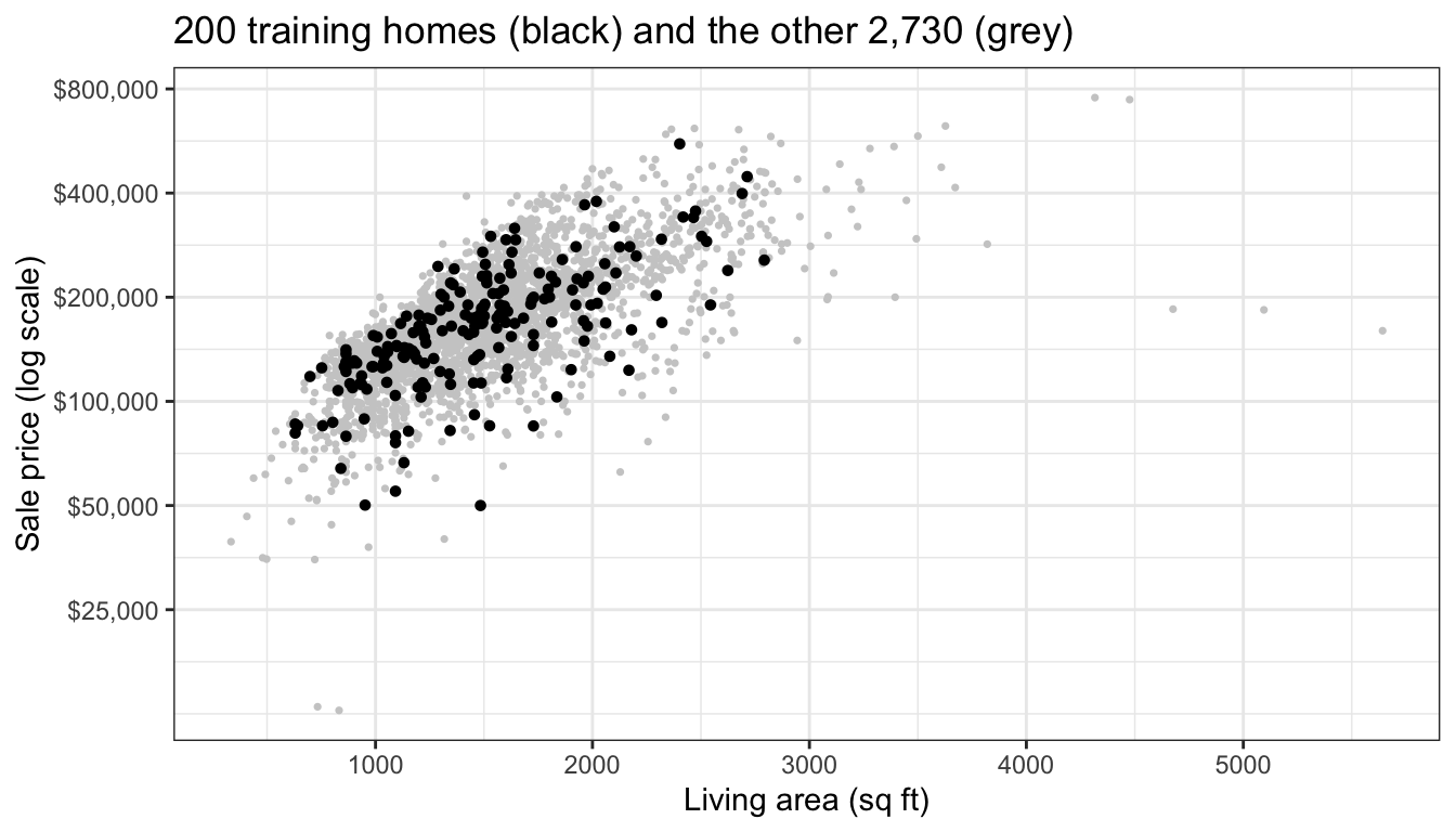

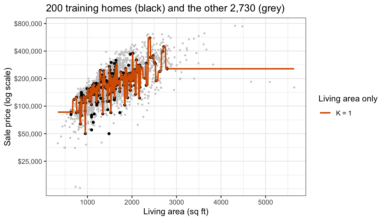
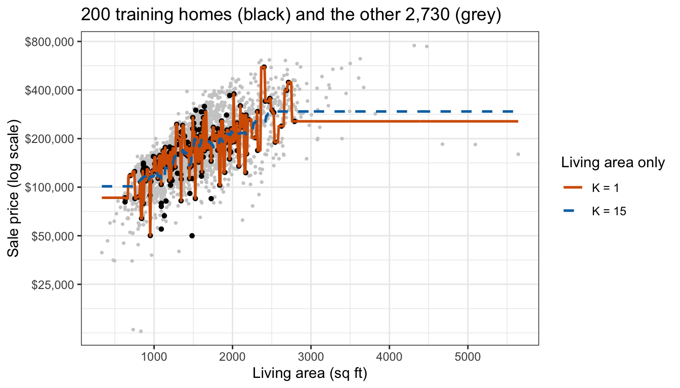
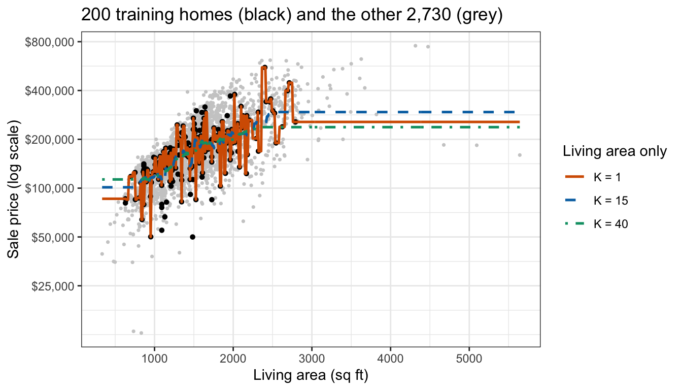
The training homes cover most of the range of living area but miss the largest homes. With $K = 1$ the fit jumps from one training home’s price to the next; with $K = 15$ and $K = 40$ it follows the trend more smoothly. All three fits are flat beyond the largest training home, at the geometric mean price (the average on the $\log_{10}$ scale) of its nearest neighbors.

18.2.1 Nested KNN candidates

The candidates are KNN regressions that differ in two tuning parameters: how many of the six explanatory variables they use, and how many neighbors. For a home with explanatory variables $x_0$,

\[\hat f_{q,K}(x_0) = \frac{1}{K}\sum_{i \in \mathcal{N}_{q,K}(x_0)} y_i,\]

where

$y_i = \log_{10}\left(\texttt{Sale\_Price}_i\right)$ is the response of training home $i$,
$p = 6$ is the number of explanatory variables available,
$q = 1, \ldots, p$ is the number used, always the first $q$ in the order listed above, so $q = 1$ is living area alone and $q = p$ adds year built, basement area, garage area, longitude, and latitude,
the features are those $q$ explanatory variables, each standardized with the mean and standard deviation of the training homes,
$\mathcal{N}_{q,K}(x_0)$ is the set of the $K$ training homes closest to $x_0$ in Euclidean distance on the (standardized) features, and
$K$ is the number of neighbors.

q_values <- seq_along(vars)
K_grid <- 1:40
candidates <- expand_grid(q = q_values, K = K_grid)
S <- nrow(candidates)
n_folds <- 10

With $K = 1, \ldots, 40$ and $q = 1, \ldots, 6$ there are $S = 240$ candidate models, indexed $s = 1, \ldots, S$. The order of the explanatory variables was chosen without using the response. Ordering them by their correlation with price in the data at hand would be another data-dependent step, and would have to be repeated inside every fold.

18.2.2 Candidate cross-validation

The function below computes the $k$-fold cross-validation estimate $\text{CV}_{(k)}$ of the test MSE, on the $\log_{10}$ scale, with $k = 10$, for all 240 candidates at once. The number of folds $k$ is unrelated to the number of neighbors $K$.

Because knn_predict() standardizes with the training folds only, standardization happens inside the folds. The choice of $q$ and $K$ does not: every candidate is fit and evaluated in every fold, and $q$ and $K$ are chosen afterward by comparing the 240 cross-validation estimates. Both steps use the training data only.

predict_candidates <- function(fit, new) {
  do.call(cbind, map(q_values, \(q) knn_predict(fit, new, q, K_grid)))
}
cv_mse <- function(data, fold) {
  predicted <- matrix(NA_real_, nrow(data), S)
  for (l in unique(fold)) {
    held_out <- fold == l
    predicted[held_out, ] <- predict_candidates(data[!held_out, ], data[held_out, ])
  }
  colMeans((data$log_price - predicted)^2)
}

18.3 Selection optimism

18.3.1 One training sample

Code

# CV estimate on the training homes and MSE on all other homes, for every
# candidate.
sample_errors <- function(train_id) {
  train <- homes[train_id, ]
  rest <- homes[-train_id, ]
  fold <- sample(rep(seq_len(n_folds), length.out = length(train_id)))
  mutate(candidates,
         cv = cv_mse(train, fold),
         test = colMeans((rest$log_price - predict_candidates(train, rest))^2))
}
one_errors <- sample_errors(one_id)
one_best <- slice_min(one_errors, cv, n = 1, with_ties = FALSE)
one_oracle <- slice_min(one_errors, test, n = 1, with_ties = FALSE)
# Candidates whose MSE on the other homes is within 5% of the smallest.
near_share <- 0.05
n_near_oracle <- sum(one_errors$test <= (1 + near_share) * one_oracle$test)

q_labels <- paste0("q = ", q_values, ": ", c("living area", "+ year built",
                   "+ basement", "+ garage", "+ longitude", "+ latitude"))
error_labels <- c("10-fold CV (training homes)", "MSE on the other homes")
one_long <- one_errors |>
  pivot_longer(c(cv, test), names_to = "error", values_to = "mse") |>
  mutate(error = factor(if_else(error == "cv", error_labels[1], error_labels[2]),
                        levels = error_labels),
         q = factor(q_labels[q], levels = q_labels))
one_marked <- one_best |>
  pivot_longer(c(cv, test), names_to = "error", values_to = "mse") |>
  mutate(error = factor(if_else(error == "cv", error_labels[1], error_labels[2]),
                        levels = error_labels),
         q = factor(q_labels[q], levels = q_labels))

curve_plot <- function(show) {
  ggplot(filter(one_long, error %in% show),
         aes(x = 1 / K, y = mse, color = error, linetype = error, shape = error)) +
    geom_line() +
    geom_point(data = filter(one_marked, error %in% show), size = 3) +
    facet_wrap(~ q, nrow = 2) +
    scale_x_log10(breaks = 1 / c(1, 5, 40), labels = c("1", "1/5", "1/40")) +
    scale_color_manual(values = setNames(c("#D55E00", "#0072B2"), error_labels),
                       drop = FALSE) +
    scale_linetype_manual(values = setNames(c("solid", "dashed"), error_labels),
                          drop = FALSE) +
    scale_shape_manual(values = setNames(c(17, 16), error_labels), drop = FALSE) +
    coord_cartesian(ylim = range(one_long$mse)) +
    labs(x = "Flexibility 1/K (log scale)", y = "MSE of log10 price",
         color = NULL, linetype = NULL, shape = NULL,
         title = paste("One sample of", m, "homes; the point marks the smallest CV estimate")) +
    theme(legend.position = "bottom")
}
one_cv_plot <- curve_plot(error_labels[1])
one_both_plot <- curve_plot(error_labels)

For the 200 training homes plotted earlier, the first tab plots the 10-fold cross-validation estimate of every candidate against the flexibility $1/K$, one panel per $q$. The remaining 2,730 homes were never used to fit or to choose, so they are test data for this sample; the second tab adds each candidate’s MSE on them.

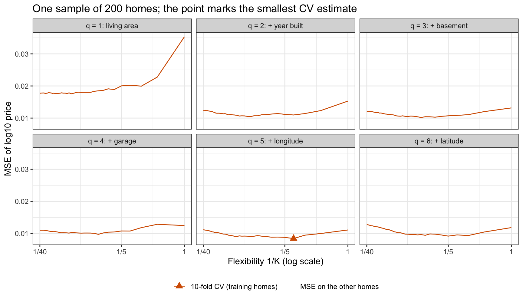
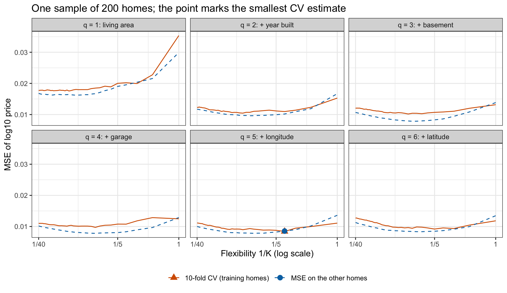
Cross-validation chooses $q = 5$ and $K = 4$, with an estimated MSE of 0.00841. Fit to the same 200 homes, that model’s MSE on the other homes is 0.00854, 1.5% above its cross-validation estimate. The candidate with the smallest MSE on the other homes is $q = 4$, $K = 9$, at 0.00780. In every panel the two curves have similar shapes, and many candidates have nearly the same MSE on the other homes: 31 of the 240 are within 5% of the smallest. In this sample the cross-validation estimate is above the MSE on the other homes for 97% of the candidates; the minimum falls where the cross-validation curve dips toward the other curve.

18.3.2 Noisy minimum

The same training homes chose the model and estimated its error. For a candidate $s$ fixed in advance,

\[\text{CV}_s = \text{MSE}^{\text{test}}_s + e_s,\]

where

$\text{CV}_s$ is the $k$-fold cross-validation estimate for candidate $s$,
$\text{MSE}^{\text{test}}_s$ is the test MSE of candidate $s$ fit to all the training homes, and
$e_s$ is the estimation error, which averages close to zero over repeated training samples (slightly above zero, since each fit in cross-validation uses $(k - 1)/k$ of the homes).

The selected candidate is $\hat s$, the one with the smallest $\text{CV}_s$, and its reported estimate is $\text{CV}_{\hat s} = \min_s \text{CV}_s$. Among candidates whose test MSEs are nearly equal, the one with the most negative $e_s$ wins, so $e_{\hat s}$ tends to be negative even though no fixed $e_s$ is.

Two candidates with equal test MSE show the size of the effect. Suppose $e_1$ and $e_2$ are jointly normal, each $N\left(0, \tau^2\right)$, with correlation $\rho$. Since $\min(a, b) = (a + b)/2 - |a - b|/2$ and $e_1 - e_2 \sim N\left[0, 2\tau^2(1 - \rho)\right]$, whose absolute value has mean $\sqrt{2\tau^2(1 - \rho)}\sqrt{2/\pi} = 2\tau\sqrt{(1 - \rho)/\pi}$,

\[E\left[\min\left(e_1, e_2\right)\right] = \frac{E\left[e_1\right] + E\left[e_2\right]}{2} - \frac{E\left[\left|e_1 - e_2\right|\right]}{2} = -\tau\sqrt{\frac{1 - \rho}{\pi}},\]

where $\tau$ is the standard deviation of each estimation error and $\rho$ the correlation between them. The optimism grows with the noise $\tau$, which is larger for smaller training samples; it shrinks as the estimates become more correlated, vanishing when $\rho = 1$; and it grows with the number of near-tied candidates, since the minimum of more noisy values is lower.

18.3.3 Repeated samples

Code

n_reps <- 300
# The QDA lecture's rule of thumb: the smallest odd integer above sqrt(n).
odd_above_sqrt <- function(n) {
  k <- floor(sqrt(n))
  if (k %% 2 == 0) k + 1 else k + 2
}
K_rule <- odd_above_sqrt(m)
procedure_labels <- c(
  paste0("Rule of thumb: q = ", max(q_values), ", K = ", K_rule, "\n(1 candidate)"),
  paste0("Best K, q = ", max(q_values), "\n(", length(K_grid), " candidates)"),
  paste0("Best K and q\n(", S, " candidates)"))
summarize_sample <- function(errors) {
  rule <- which(errors$q == max(q_values) & errors$K == K_rule)
  all_six <- which(errors$q == max(q_values))
  best_K <- all_six[which.min(errors$cv[all_six])]
  best_all <- which.min(errors$cv)
  chosen <- c(rule, best_K, best_all)
  tibble(procedure = procedure_labels, q = errors$q[chosen], K = errors$K[chosen],
         cv = errors$cv[chosen], test = errors$test[chosen])
}
optimism <- map(seq_len(n_reps), \(r) {
  summarize_sample(sample_errors(sample(n_homes, m))) |> mutate(rep = r)
}) |>
  list_rbind() |>
  mutate(procedure = factor(procedure, levels = procedure_labels),
         gap = cv - test,
         relative_gap = gap / test)
optimism_summary <- optimism |>
  group_by(procedure) |>
  summarize(mean_gap = mean(gap), mean_relative = mean(relative_gap),
            se_relative = sd(relative_gap) / sqrt(n()),
            share_below = mean(gap < 0), mean_test = mean(test),
            .groups = "drop")
opt_of <- function(i, col) optimism_summary[[col]][i]
# "x% below" or "x% above" for the average relative gap of procedure i.
gap_text <- function(i) {
  g <- opt_of(i, "mean_relative")
  paste(pct(abs(g)), if (g < 0) "below" else "above")
}

optimism_plot <- ggplot(optimism, aes(x = procedure, y = 100 * relative_gap)) +
  geom_hline(yintercept = 0, linetype = "dashed") +
  geom_violin(fill = "grey90", scale = "width", quantiles = c(0.25, 0.5, 0.75),
              quantile.linetype = "solid") +
  stat_summary(fun = mean, geom = "point", shape = 23, size = 3,
               fill = "#E69F00") +
  labs(x = NULL, y = "CV estimate minus test MSE\n(% of test MSE)",
       title = paste(n_reps, "training samples of", m, "homes"),
       caption = "Lines = quartiles and median, diamond = mean, dashed line = no gap.")

One sample can be lucky or unlucky. To see what happens on average, a training sample of 200 homes was drawn 300 times. In each sample, three procedures chose a model by 10-fold cross-validation, and the chosen model’s cross-validation estimate was compared with its MSE on the other 2,730 homes:

rule of thumb: one candidate fixed in advance, all six explanatory variables with $K = 15$, the smallest odd integer above $\sqrt{200}$ (the QDA lecture’s rule of thumb), so nothing is chosen,
best $K$: the smallest estimate among the 40 values of $K$ with all six explanatory variables, and
best $K$ and $q$: the smallest estimate among all 240 candidates.

The figure shows, for each procedure, the distribution over samples of the gap between the chosen model’s cross-validation estimate and its test MSE, as a percentage of the test MSE. A negative gap means the estimate was too optimistic.

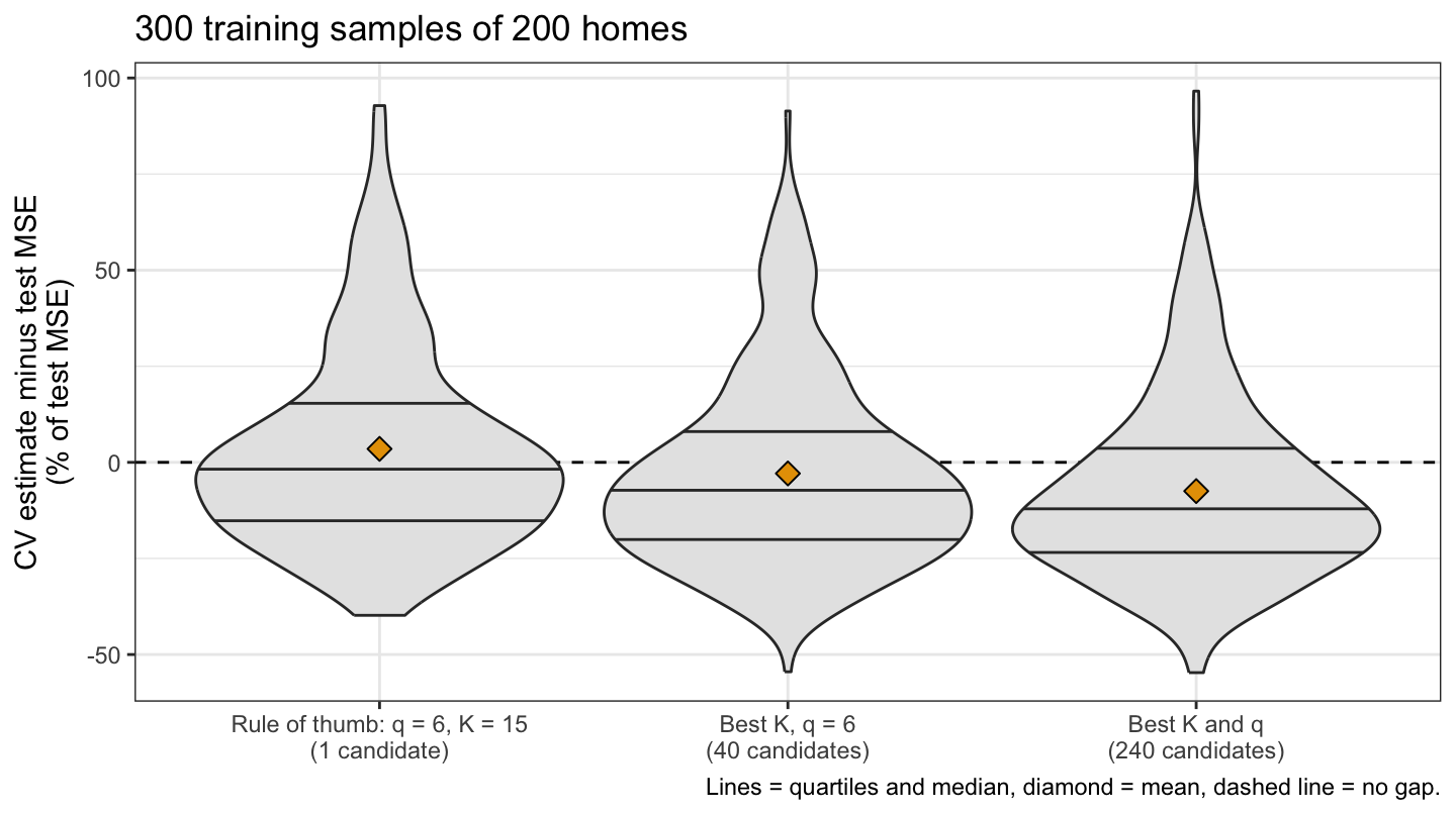
For the rule of thumb, which chooses nothing, the cross-validation estimate averages 3.5% above the test MSE (simulation standard error 1.5 percentage points) and falls below it in 53% of samples. The best of 40 values of $K$ averages 2.9% below, and the best of all 240 candidates 7.5% below (standard error 1.4 percentage points), below the test MSE in 70% of samples.

The choosing also gains something real: the average test MSE of the model chosen from all 240 candidates is 0.00811, against 0.00874 for the rule of thumb. On these data the optimism is modest. By the two-candidate calculation above, it would be larger with smaller training samples, whose estimates are noisier, or with more near-tied candidates whose estimates are less correlated.

18.4 Test data workflow

test_share <- 0.2
test_id <- sample(n_homes, round(test_share * n_homes))
train <- homes[-test_id, ]
test <- homes[test_id, ]

In practice there is one data set, not a population to resample from. The figure splits the 2,930 homes at random into 2,344 training homes (blue circles) and 586 test homes (orange triangles), 20% of the total.

Code

set_labels <- c("Training", "Test")
split_plot <- homes |>
  mutate(set = factor(if_else(row_number() %in% test_id, "Test", "Training"),
                      levels = set_labels)) |>
  arrange(set) |>
  ggplot(aes(x = Gr_Liv_Area, y = Sale_Price, color = set, shape = set)) +
  geom_point(alpha = 0.6, size = 1) +
  scale_color_manual(values = c(Training = "#0072B2", Test = "#E69F00")) +
  scale_shape_manual(values = c(Training = 16, Test = 17)) +
  price_axis +
  labs(x = "Living area (sq ft)", y = "Sale price (log scale)", color = NULL,
       shape = NULL, title = "modeldata::ames, one random split")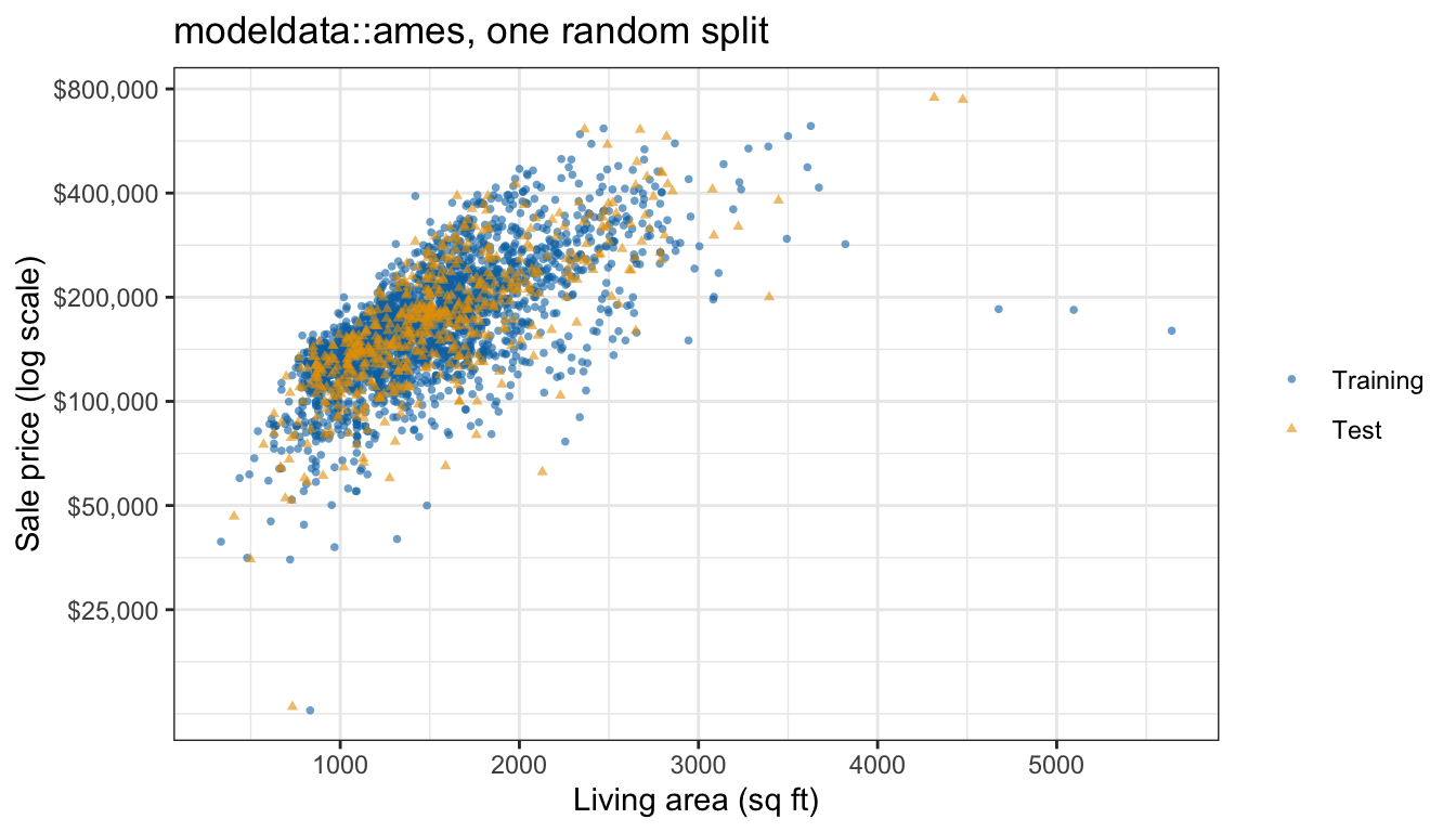

The two sets overlap over the bulk of the data. Of the 5 homes with more than 4,000 square feet, 2 are in the test set.

18.4.1 Workflow steps

The simulation shows that when the same data choose a model and estimate its error, the estimate is optimistic on average. The remedy is to keep some data out of the choosing entirely:

Split off test data first, at random, before any plotting, fitting, or choosing.
Choose by cross-validation on the training data only. Every data-dependent step of fitting is repeated inside each fold using only the training folds: here standardization, computed inside knn_predict(). The held-out folds are validation sets. Feature selection (the number $q$ of explanatory variables) and tuning ($K$) are done by comparing the cross-validation estimates of all the candidates, so they also use the training data only, and the smallest estimate tends to be optimistic.
Refit the chosen model to all the training data.
Evaluate it once on the test data, and report that test MSE as the estimate of its error on new homes.

18.4.2 Choosing

Code

train_fold <- sample(rep(seq_len(n_folds), length.out = nrow(train)))
final_errors <- mutate(candidates, cv = cv_mse(train, train_fold))
final_best <- slice_min(final_errors, cv, n = 1, with_ties = FALSE)
final_min_by_q <- final_errors |>
  group_by(q) |>
  summarize(cv = min(cv), .groups = "drop")

final_cv_plot <- final_errors |>
  mutate(q = factor(q_labels[q], levels = q_labels)) |>
  ggplot(aes(x = 1 / K, y = cv)) +
  geom_line(color = "#D55E00") +
  geom_point(data = mutate(final_best, q = factor(q_labels[q], levels = q_labels)),
             color = "#D55E00", shape = 17, size = 3) +
  facet_wrap(~ q, nrow = 2) +
  scale_x_log10(breaks = 1 / c(1, 5, 40), labels = c("1", "1/5", "1/40")) +
  labs(x = "Flexibility 1/K (log scale)", y = "10-fold CV estimate of MSE\n(log10 price)",
       title = paste(format(nrow(train), big.mark = ","),
                     "training homes; the triangle marks the minimum"))

The figure plots the 10-fold cross-validation estimate of each of the 240 candidates on the 2,344 training homes.

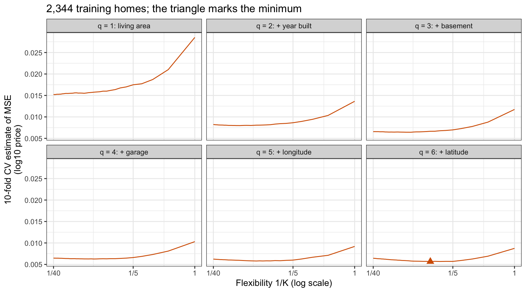
With 2,344 training homes the curves are smoother than for the sample of 200. Each curve rises steeply toward $K = 1$. The smallest estimate in each panel is 0.0152, 0.0080, 0.0064, 0.0063, 0.0058, and 0.0057 for $q = 1$ through 6: year built gives by far the largest improvement and basement area the next largest, while the last three explanatory variables lower it only slightly. Cross-validation chooses $q = 6$ and $K = 9$, with an estimated MSE of 0.00567.

18.4.3 Final evaluation

final_pred <- knn_predict(train, test, final_best$q, final_best$K)
final_test_mse <- mean((test$log_price - final_pred)^2)

Code

test_errors <- test$log_price - final_pred
test_big <- test$Gr_Liv_Area > big_area
final_test_mse_small <- mean(test_errors[!test_big]^2)
big_pred_price <- 10^final_pred[test_big]
big_price <- test$Sale_Price[test_big]
# Standard error of the test MSE, a mean of nrow(test) squared errors.
final_test_se <- sd(test_errors^2) / sqrt(nrow(test))
# Share of test homes predicted within the root-mean-square factor.
final_rmse <- sqrt(final_test_mse)
within_rmse <- mean(abs(test_errors) < final_rmse)
# For illustration only, outside the workflow: every candidate's test MSE.
hindsight <- mutate(final_errors,
                    test = colMeans((test$log_price - predict_candidates(train, test))^2))
hindsight_best <- slice_min(hindsight, test, n = 1, with_ties = FALSE)
# Relative gap between the test MSE and the CV estimate, as a % of the CV estimate.
rel_gap <- function(test_mse, cv) {
  paste(pct(abs(test_mse / cv - 1), 0), if (test_mse > cv) "above" else "below")
}

Refit to all 2,344 training homes and used once on the 586 test homes, the chosen model has a test MSE of 0.00641, against its cross-validation estimate of 0.00567. The root mean squared error is 0.080 on the $\log_{10}$ scale. An error of $e$ on that scale is a factor of $10^e$ in price, so the root-mean-square error is a factor of $10^{0.080} = 1.20$, too high or too low; 81% of the test homes are predicted within that factor.

The test MSE is 13% above the cross-validation estimate. Selection optimism is at most a modest part of this gap. In the simulation, the smallest of 240 estimates averaged 7.5% below the test MSE with 200 training homes; with 2,344 training homes each estimate is less noisy, so the optimism should be smaller. Choosing differently would not have closed the gap either: for illustration only, outside the workflow, the candidate with the smallest MSE on these test homes, $q = 6$ and $K = 8$, has a test MSE only 0.8% below the chosen model’s.

Part of the gap comes from the 2 test homes with more than 4,000 square feet, which sold for $755,000 and $745,000 and were predicted at $446,000 and $446,000, the geometric mean price (the average on the $\log_{10}$ scale) of the nearest training homes; without them the test MSE is 0.00626, 10% above the cross-validation estimate. The standard error of a mean of 586 squared errors is 0.00137, 21% of the test MSE, so the gap is smaller than the variability of an MSE computed from 586 homes. The test MSE is the number to report: no choice was made with the test homes, so the selection optimism of the previous section does not affect it.

The test data can be used only once: if the test MSE were used to choose again, for example by going back to try another $q$ after seeing it, the test homes would become one more validation set, and the reported error would be the minimum over the choices tried, with the same optimism as the minimum of the cross-validation curve.

Beyond this course

One-standard-error rule. When the cross-validation curve is flat near its minimum, as in several panels above, choose the simplest candidate (the largest $K$, or the smallest $q$) whose estimate is within one standard error of the minimum. It trades a little estimated error for a model less tuned to the noise in this particular sample.
Nested cross-validation. When the data are too few to set aside test data, an outer cross-validation loop around the whole procedure (“choose $q$ and $K$ by inner cross-validation, then refit”) estimates the test error of that procedure, using every observation for both choosing and testing, but never in the same loop.

18.5 Activity

In small groups, work through 15-cv-in-practice_activity.R (download) in RStudio. It uses modeldata::stackoverflow, responses from 5,594 developers to Stack Overflow’s annual Developer Survey, to ask which developers work remotely; the response variable is Remote, whether or not the developer works remotely. Your group splits off test data, looks at the training data, compares logistic regression, LDA, and KNN with several values of $K$ by 10-fold cross-validation on the training data, chooses one, and evaluates it once on the test data. The classifiers are compared mainly by the area under the ROC curve (AUC) and also by the error rate, each against the benchmark of always predicting “Not remote,” whose AUC is 0.5. Most of the code is provided; the discussion questions at the end of the script are the point of the activity.

18.6 Conclusion

Cross-validation estimates the test error of a model fixed in advance with little bias. Once it is used to choose among candidate models, its minimum is no longer such an estimate. The same data choose the model and estimate its error, so the candidate that wins is the one whose estimate happened to fall lowest, and the winning estimate tends to be below the chosen model’s test error. The optimism grows with the number of nearly equivalent candidates and with the noise in their estimates, and shrinks when the estimates are strongly correlated.

The remedy is a division of labor among the three roles of data. Test data are split off first and set aside. All choosing happens by cross-validation on the training data only. Every data-dependent step of fitting, such as standardization, is repeated inside each fold, so that the held-out folds serve as validation sets; features and tuning parameters are then chosen by comparing the cross-validation estimates of the candidates, and the smallest of those estimates tends to be optimistic. The chosen model is refit to all the training data and evaluated once on the test data, and that test error is what gets reported. Using the test data to choose again turns them into validation data and brings the optimism back.

The next lecture begins Chapter 6, linear model selection and regularization, with subset selection. The bootstrap chapter that follows this one in the book is optional reading.