23 Principal Components

Learning objectives

After this lecture you should be able to

define the loading vector $\phi_1$ and the scores $z_{i1}$ of the first principal component, and derive $\phi_1$ as the eigenvector of the sample correlation matrix with the largest eigenvalue, by maximizing the sample variance of the scores subject to $\left\|\phi_1\right\| = 1$,
explain why the first principal component is also the line closest to the standardized data, in average squared distance,
describe the later components as orthogonal directions of decreasing variance, compute the proportion of variance explained by each component and cumulatively, and choose a number of components $M$ from a scree plot or a cumulative rule, stating why the choice is a judgment,
explain why the features are standardized before principal component analysis, and predict which explanatory variable dominates the first component when they are not,
interpret the loadings and scores of a component, including why the sign of a loading vector is arbitrary, and
explain why principal component analysis is unsupervised, why it is not variable selection, and why the component with the most variance need not be the best predictor of a response.

Subset selection, ridge regression, and the lasso fit a model to all $p$ features and control its flexibility by keeping some of the features or by shrinking the coefficient estimates. Dimension reduction instead replaces the $p$ features by $M < p$ linear combinations of them and fits a model to those. Here $M$ is the number of components kept; in the ridge and lasso lectures it was the number of repeated training samples. This lecture constructs the linear combinations, the principal components; the next one regresses on them. Principal component analysis is the subject of ISLR2 Chapter 12, which the course reaches after Exam 2.

23.1 Diamond measurements

23.1.1 Data

Question. Diamonds are described by six numbers: weight, two proportions, and three physical dimensions. Can fewer than six directions capture most of the variation in these numbers?

Data. ggplot2::diamonds records 53,940 diamonds. The response variable is the price, price, in US dollars, which this lecture does not use. The numeric explanatory variables are

carat, the weight (one carat is 200 mg),
depth, the total depth percentage, the height of the diamond as a percentage of its average width, $100z/\left[(x + y)/2\right]$, computed from the three dimensions below,
table, the width of the flat top facet as a percentage of the widest point, and
x, y, and z, the length, width, and depth in mm.

cut, color, and clarity are ordered categories with no numeric scale, so they have no variance or correlation in the sense used below and are left out.

23.1.2 Recording errors

The figure plots the width y and the depth z against the length x for all 53,940 diamonds.

Code

# The numeric explanatory variables, and the largest plausible dimension.
features <- c("carat", "depth", "table", "x", "y", "z")
max_mm <- 20

# Flag diamonds with a zero dimension or a dimension above max_mm.
status_levels <- c("Kept", "Removed")
diamonds_flagged <- diamonds |>
  mutate(zero = x == 0 | y == 0 | z == 0,
         extreme = !zero & (x > max_mm | y > max_mm | z > max_mm),
         status = if_else(zero | extreme, "Removed", "Kept"),
         status = factor(status, levels = status_levels))

# Zero dimensions, and diamonds removed for each reason.
n_zero <- c(x = sum(diamonds$x == 0),
            y = sum(diamonds$y == 0),
            z = sum(diamonds$z == 0))
n_zero_rows <- sum(diamonds_flagged$zero)
n_extreme <- sum(diamonds_flagged$extreme)

# The retained diamonds, their number n, and the number of features p.
kept <- diamonds_flagged |>
  filter(status == "Kept") |>
  select(-zero, -extreme, -status)
n <- nrow(kept)
p <- length(features)
largest_kept <- max(kept[c("x", "y", "z")])

# Dimensions above max_mm, and the other dimensions of those diamonds.
dims <- as.matrix(diamonds[c("x", "y", "z")])
n_big_values <- sum(dims > max_mm)
big_rows <- dims[diamonds_flagged$extreme, , drop = FALSE]
big_others <- big_rows[big_rows <= max_mm]
big_widths <- sort(diamonds$y[diamonds$y > max_mm], decreasing = TRUE)

# Width and depth against length, one panel each, removed diamonds on top.
dimension_labels <- c("Width y (mm)", "Depth z (mm)")
n_diamonds <- nrow(diamonds)
cleaning_title <- paste(big(n_diamonds), "diamonds")
cleaning_plot <- diamonds_flagged |>
  pivot_longer(c(y, z), names_to = "dimension", values_to = "value") |>
  mutate(dimension = if_else(dimension == "y",
                             "Width y (mm)",
                             "Depth z (mm)"),
         dimension = factor(dimension, levels = dimension_labels)) |>
  arrange(status) |>
  ggplot(aes(x = x, y = value, color = status, shape = status)) +
  geom_point(alpha = 0.6, size = 1) +
  facet_wrap(~ dimension) +
  scale_color_manual(values = c("grey40", "#D55E00")) +
  scale_shape_manual(values = c(16, 17)) +
  labs(x = "Length x (mm)",
       y = NULL,
       color = NULL,
       shape = NULL,
       title = cleaning_title) +
  theme(legend.position = "bottom")

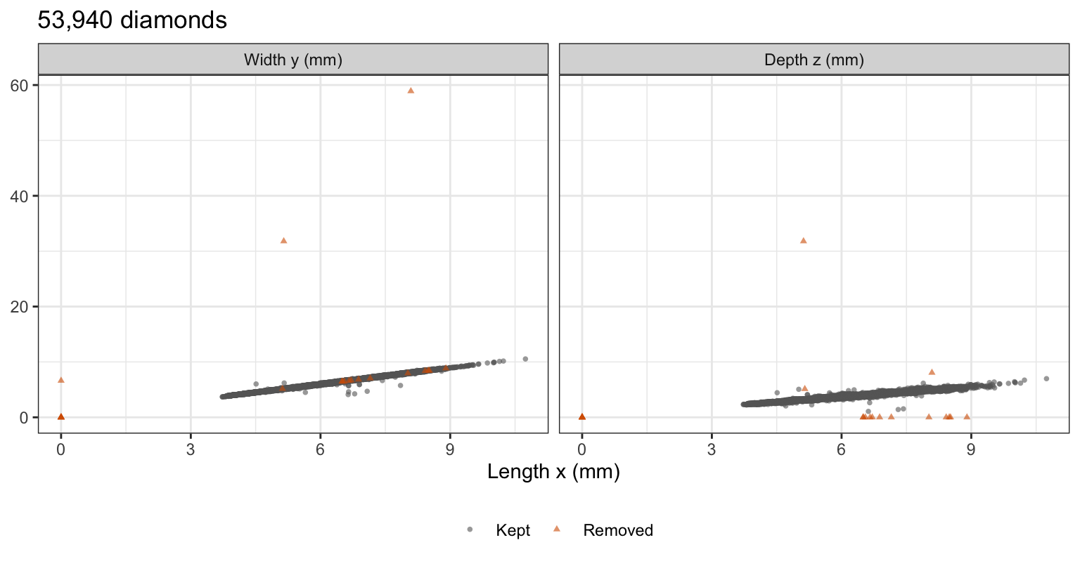
Most diamonds lie close to the line width = length, and depth rises with length. 8 diamonds have length 0, 7 width 0, and 20 depth 0, 20 diamonds in all; a physical dimension of 0 mm is impossible. There are 3 values above 20 mm: widths of 58.9 and 31.8 mm and a depth of 31.8 mm, on diamonds whose other dimensions are 5.12 to 8.09 mm. A handful of other diamonds sit away from the cloud, below it in the depth panel, but their values are possible.

The rule used here removes every diamond with a dimension of 0 or larger than 20 mm: 23 diamonds (20 with a zero, 3 with an extreme value), leaving $n = 53{,}917$. The largest remaining dimension is 10.74 mm. Every computation below uses all $n$ retained diamonds; the scatterplots show a random subsample of them.

23.1.3 Correlated measurements

# Retained diamonds drawn at random for the scatterplots.
n_sub <- 1000
sub_id <- sample(n, n_sub)

# The number of them shown in the two-feature figures.
n_shown <- 250

The lower panels of the scatterplot matrix plot each pair of explanatory variables for 1,000 diamonds drawn at random from the retained ones, the first random draw after set.seed(20261021). The upper panels give the correlations over all $n$ retained diamonds.

Code

# Explanatory variables as a matrix, their correlations, and the subsample.
X <- as.matrix(kept[features])
cor_X <- cor(X)
X_sub <- X[sub_id, ]

# Plot titles for all retained diamonds and for the subsample.
title_all <- paste(big(n), "retained diamonds")
title_sub <- paste(big(n_sub), "retained diamonds")

# Midpoint of each variable's range in the subsample, where text is placed.
sub_min <- apply(X_sub, 2, min)
sub_max <- apply(X_sub, 2, max)
mid <- (sub_min + sub_max) / 2

# Panel column and row variables as factors, in the order of features.
as_grid <- function(d) {
  mutate(d,
         xvar = factor(xvar, levels = features),
         yvar = factor(yvar, levels = features))
}

# Lower panels: the subsampled points of each pair of variables.
pair_index <- combn(p, 2)
pair_points <- function(k) {
  first <- pair_index[1, k]
  second <- pair_index[2, k]
  tibble(xvar = features[first],
         yvar = features[second],
         xval = X_sub[, first],
         yval = X_sub[, second])
}
n_pairs <- ncol(pair_index)
lower <- map(seq_len(n_pairs), pair_points) |>
  list_rbind() |>
  as_grid()

# Upper panels: the correlation over all n retained diamonds.
upper_x <- features[pair_index[2, ]]
upper_y <- features[pair_index[1, ]]
upper_r <- cor_X[cbind(upper_x, upper_y)]
upper <- tibble(xvar = upper_x,
                yvar = upper_y,
                xval = mid[upper_x],
                yval = mid[upper_y],
                label = fmt_math(upper_r)) |>
  as_grid()

# Diagonal panels: each carries its variable's range, so every row and
# column has a scale, and its name and unit.
diagonal_points <- function(f) {
  tibble(xvar = f, yvar = f, xval = X_sub[, f], yval = X_sub[, f])
}
diagonal <- map(features, diagonal_points) |>
  list_rbind() |>
  as_grid()
units <- c(carat = "carats",
           depth = "%",
           table = "%",
           x = "mm",
           y = "mm",
           z = "mm")
diagonal_text <- tibble(xvar = features,
                        yvar = features,
                        xval = mid,
                        yval = mid,
                        label = paste0(features, "\n(", units, ")")) |>
  as_grid()

# Scatterplot matrix: points below the diagonal, correlations above it.
pairs_caption <- paste("Upper panels: correlations over all",
                       big(n),
                       "retained diamonds.")
pairs_plot <- ggplot(lower, aes(x = xval, y = yval)) +
  geom_point(alpha = 0.3, size = 0.5) +
  geom_blank(data = diagonal) +
  geom_text(data = upper, aes(label = label), size = 5) +
  geom_text(data = diagonal_text,
            aes(label = label),
            size = 4,
            fontface = "bold") +
  facet_grid(yvar ~ xvar, scales = "free", switch = "both") +
  labs(x = NULL,
       y = NULL,
       title = title_sub,
       caption = pairs_caption) +
  theme(strip.placement = "outside",
        axis.text = element_text(size = 7))

# Correlations among the four size variables, and of depth and table with
# them.
size_vars <- c("carat", "x", "y", "z")
size_cors <- cor_X[size_vars, size_vars][upper.tri(diag(4))]
other_cors <- cor_X[c("depth", "table"), size_vars]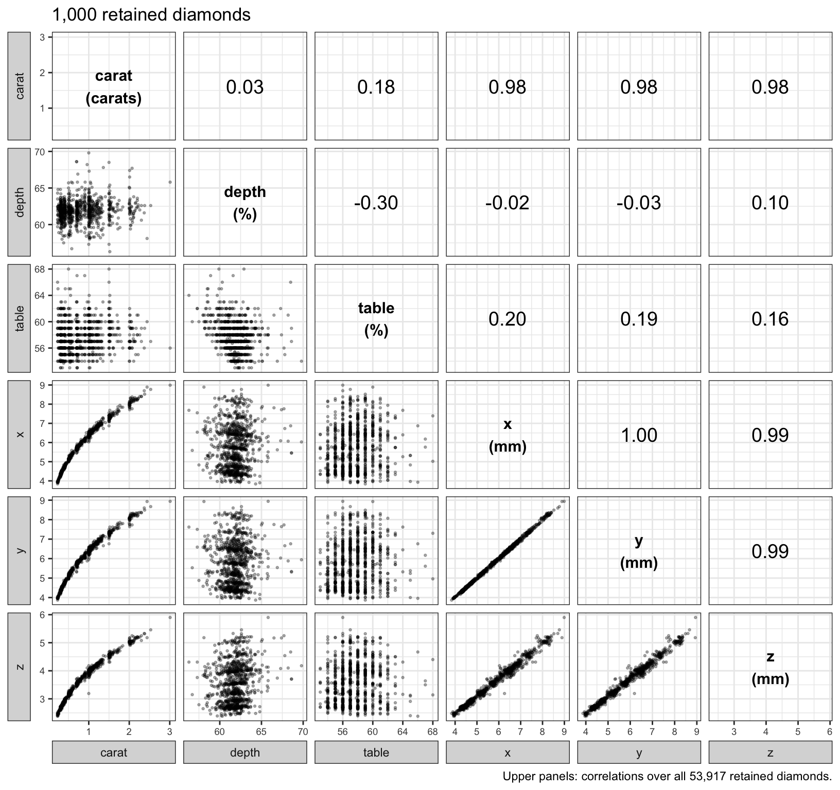

Carat, length, width, and depth in mm rise together: their correlations are 0.98 to 1.00. Length, width, and depth are close to linear in one another, and carat curves upward against each of them, since weight grows with volume. Depth percentage and table are nearly unrelated to these four (correlations −0.03 to 0.20) and weakly to each other (−0.30). Four of the six explanatory variables are close to one measurement, the size of the diamond.

Depth percentage is not a separate measurement.

# Recorded depth percentage against the one computed from the dimensions.
average_width <- (kept$x + kept$y) / 2
depth_computed <- 100 * kept$z / average_width
depth_gap <- abs(kept$depth - depth_computed)

Over the $n$ retained diamonds, recorded depth differs from $100z/\left[(x + y)/2\right]$ by a median of 0.03 percentage points, the size of the rounding in the recorded values; only 77 diamonds differ by more than 1 point, the largest by 44.5 points. The six explanatory variables therefore carry five measurements: weight, table, and the three dimensions. Depth percentage is nearly uncorrelated with size because it records the depth z relative to x and y, a shape, not a size.

23.1.4 Features

The features are the standardized explanatory variables,

\[\tilde x_{ij} = \frac{x_{ij} - \bar x_j}{s_j}, \qquad s_j = \sqrt{\frac{1}{n}\sum_{i=1}^n\left(x_{ij} - \bar x_j\right)^2},\]

where

$x_{ij}$ is explanatory variable $j = 1, \ldots, p$ of diamond $i = 1, \ldots, n$, in the order carat, depth, table, x, y, and z, so $p = 6$,
$\bar x_j$ and $s_j$ are the mean and the standard deviation (divisor $n$) of explanatory variable $j$, as in the Ridge Regression lecture, and
$\tilde x_{ij}$ is feature $j$ of diamond $i$; $\tilde{\mathbf{X}}$ is the $n \times p$ matrix of features and $\tilde x_i$ its row $i$.

Each feature has mean 0 and $\frac{1}{n}\sum_i\tilde x_{ij}^2 = 1$, and

\[\mathbf{R} = \frac{1}{n}\tilde{\mathbf{X}}^\top\tilde{\mathbf{X}}\]

is the $p \times p$ sample correlation matrix, whose entries are the upper panels of the scatterplot matrix. The bold $\mathbf{R}$ is a matrix and is unrelated to the coefficient of determination $R^2$, which appears once, in the section on price. The section on scaling shows what happens without standardization.

# Standard deviation with divisor n.
sd_n <- function(v) {
  deviations <- v - mean(v)
  sqrt(mean(deviations^2))
}

# Standardized features and their correlation matrix R.
X_std <- scale(X, center = TRUE, scale = apply(X, 2, sd_n))
R <- crossprod(X_std) / n

23.2 First principal component

23.2.1 Two features

The first figure plots standardized table against standardized depth for the first 250 diamonds of the subsample. The other tabs add a direction through the origin and each diamond’s perpendicular projection onto it.

Code

# Standardized depth and table, and their correlation.
X_dt <- X_std[, c("depth", "table")]
r_dt <- cor_X["depth", "table"]

# Unit direction at angle theta, in degrees from the depth axis.
direction <- function(theta) {
  radians <- theta * pi / 180
  c(cos(radians), sin(radians))
}

# Variance, over all n diamonds, of the scores along direction theta.
score_variance <- function(theta) {
  mean((X_dt %*% direction(theta))^2)
}

# For each angle: the variance of the scores and the mean squared distance
# to the line.
theta_grid <- 0:180
mean_sq_length <- mean(rowSums(X_dt^2))
theta_curves <- tibble(theta = theta_grid,
                       variance = map_dbl(theta_grid, score_variance),
                       distance = mean_sq_length - variance)
theta_best <- theta_curves$theta[which.max(theta_curves$variance)]

# Value of one column of theta_curves at one angle.
at_theta <- function(theta, col) {
  theta_curves[[col]][theta_curves$theta == theta]
}

# Base plot: the first n_shown diamonds of the subsample.
shown <- as_tibble(X_dt[sub_id[seq_len(n_shown)], ])
dt_caption <- paste("Variance and mean squared distance over all",
                    big(n),
                    "retained diamonds.")
dt_base <- ggplot(shown, aes(x = depth, y = table)) +
  coord_equal(xlim = c(-4, 4), ylim = c(-4, 4)) +
  labs(x = "Standardized depth",
       y = "Standardized table",
       title = paste(n_shown, "retained diamonds"),
       caption = dt_caption)

# The line at angle theta and each diamond's projection onto it.
dt_projection <- function(theta) {
  a <- direction(theta)
  proj <- mutate(shown,
                 score = depth * a[1] + table * a[2],
                 depth_p = score * a[1],
                 table_p = score * a[2])
  variance <- fmt(at_theta(theta, "variance"))
  distance <- fmt(at_theta(theta, "distance"))
  subtitle <- paste0("Angle ",
                     theta,
                     " degrees: score variance ",
                     variance,
                     ", mean squared distance ",
                     distance)
  dt_base +
    geom_abline(slope = a[2] / a[1],
                intercept = 0,
                color = "#D55E00",
                linewidth = 0.9) +
    geom_segment(data = proj,
                 aes(xend = depth_p, yend = table_p),
                 color = "#0072B2",
                 alpha = 0.5) +
    geom_point(alpha = 0.5, size = 1) +
    labs(subtitle = subtitle)
}

# Tabs: the data, the depth axis, and the first principal component.
dt_data <- dt_base +
  geom_point(alpha = 0.5, size = 1) +
  labs(caption = NULL)
dt_plots <- list(dt_data,
                 dt_projection(0),
                 dt_projection(theta_best))

# Both quantities against the angle, the two angles above dotted.
theta_title <- paste(big(n), "retained diamonds, standardized depth and table")
theta_plot <- theta_curves |>
  pivot_longer(-theta, names_to = "quantity") |>
  mutate(quantity = if_else(quantity == "variance",
                            "Variance of the scores",
                            "Mean squared distance to the line")) |>
  ggplot(aes(x = theta, y = value, color = quantity, linetype = quantity)) +
  geom_vline(xintercept = c(0, theta_best),
             color = "grey60",
             linetype = "dotted") +
  geom_line(linewidth = 0.9) +
  scale_color_manual(values = okabe_ito[c(4, 5)]) +
  scale_x_continuous(breaks = seq(0, 180, by = 45)) +
  labs(x = "Angle of the direction (degrees from the depth axis)",
       y = NULL,
       color = NULL,
       linetype = NULL,
       title = theta_title) +
  theme(legend.position = "bottom")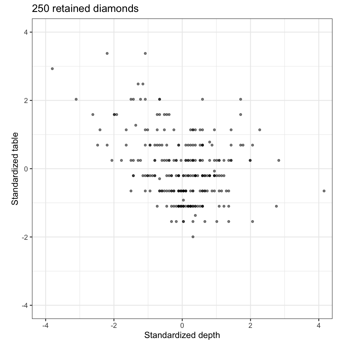

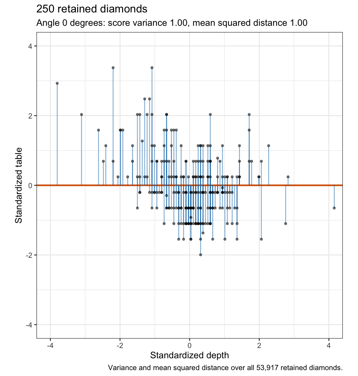
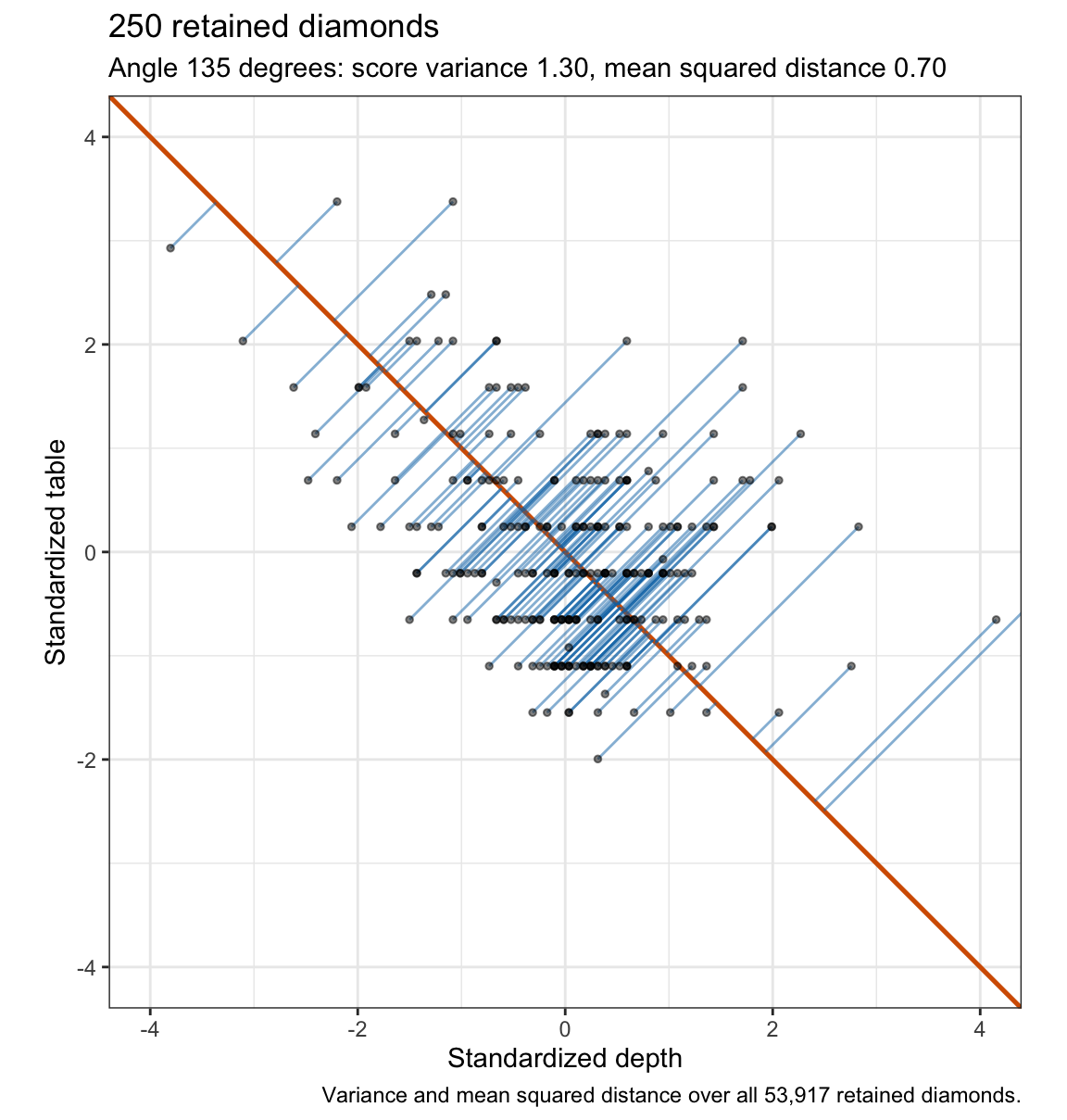
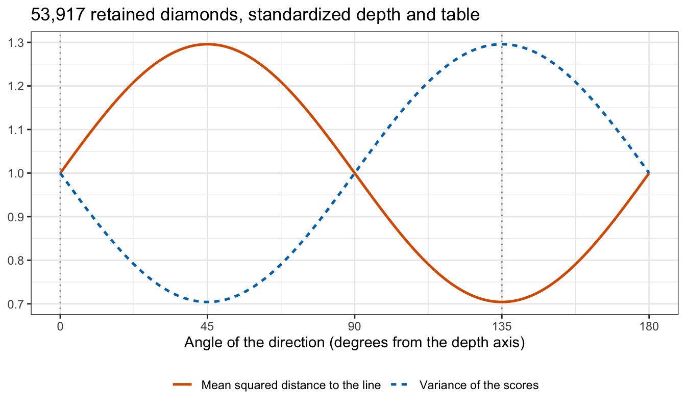
The cloud is tilted down to the right, the negative correlation $r = -0.30$ between depth and table. Projected onto the depth axis, the diamonds’ positions along the line have variance 1.00, the variance of standardized depth. Along the line at 135 degrees, which runs with the tilt, they spread more, variance 1.30, and the projection segments are shorter. The last tab sweeps the direction through every angle: the variance of the positions along the line is largest at the same angle at which the mean squared distance to the line is smallest.

23.2.2 Loadings and scores

The first principal component of the features is the linear combination

\[Z_1 = \phi_{11}\tilde X_1 + \phi_{21}\tilde X_2 + \cdots + \phi_{p1}\tilde X_p, \qquad \sum_{j=1}^p\phi_{j1}^2 = 1,\]

with the largest sample variance, where

$\tilde X_j$ is feature $j$, the standardized explanatory variable,
$\phi_{j1}$ is the loading of feature $j$ on the first component, and $\phi_1 = \left(\phi_{11}, \ldots, \phi_{p1}\right)^\top$ is the loading vector, a unit-length direction in the $p$-dimensional feature space (not the dispersion parameter $\phi$ of the Generalized Linear Models lecture), and
the value of $Z_1$ for diamond $i$,

\[z_{i1} = \sum_{j=1}^p\phi_{j1}\tilde x_{ij} = \tilde x_i\phi_1,\]

is its score on the first component, its signed position along the direction $\phi_1$. The $n$-vector of scores is $z_1 = \tilde{\mathbf{X}}\phi_1$.

Without the constraint $\left\|\phi_1\right\| = 1$ the variance could be made as large as desired by multiplying the loadings by a constant. In the two-feature figure, the line at angle $\theta$ has unit direction $a = \left(\cos\theta, \sin\theta\right)^\top$, each blue segment ends at the projection $\left(\tilde x_ia\right)a^\top$ of a diamond onto it, and the first component is the line with the largest variance of $\tilde x_ia$.

23.2.3 Maximum variance

The features have mean 0, so the scores of any unit vector $a$ have mean 0 and sample variance

\[\frac{1}{n}\sum_{i=1}^n\left(\tilde x_i a\right)^2 = \frac{1}{n}a^\top\tilde{\mathbf{X}}^\top\tilde{\mathbf{X}}a = a^\top\mathbf{R}a.\]

To maximize $a^\top\mathbf{R}a$ subject to $a^\top a = 1$, introduce a Lagrange multiplier $v$ and set the gradient of $a^\top\mathbf{R}a - v\left(a^\top a - 1\right)$ to zero:

\[2\mathbf{R}a - 2va = 0 \quad\Rightarrow\quad \mathbf{R}a = va.\]

So a maximizing direction is an eigenvector of $\mathbf{R}$ with eigenvalue $v$, and multiplying $\mathbf{R}a = va$ on the left by $a^\top$ shows that the variance of its scores is $a^\top\mathbf{R}a = va^\top a = v$. Of all the unit eigenvectors, the one with the largest eigenvalue gives the largest variance: $\phi_1$ is the eigenvector of the sample correlation matrix with the largest eigenvalue $v_1$, and $v_1$ is the variance of the first component’s scores. Both are estimates, computed from the $n$ diamonds, of the leading eigenvector and eigenvalue of the population correlation matrix of the explanatory variables.

For two features, $\mathbf{R} = \left[\begin{smallmatrix}1 & r\\ r & 1\end{smallmatrix}\right]$ and

\[a^\top\mathbf{R}a = \cos^2\theta + \sin^2\theta + 2r\cos\theta\sin\theta = 1 + r\sin 2\theta.\]

With $r < 0$ it is largest at $\theta = 135$ degrees, where it equals $1 + |r| = 1.30$: the eigenvalues of $\mathbf{R}$ are $1 \pm r$, with eigenvectors $\left(1, 1\right)^\top/\sqrt 2$ and $\left(1, -1\right)^\top/\sqrt 2$. For two standardized features with $r \ne 0$, the first principal component is always one of the two 45-degree lines; the correlation decides which one and how much variance it carries. With $r = 0$ the eigenvalues tie and every direction is a first component.

23.2.4 Closest line

Because $\phi_1$ has unit length, Pythagoras splits each diamond’s squared distance from the origin into its squared score and its squared distance from the line:

\[\left\|\tilde x_i\right\|^2 = z_{i1}^2 + \left\|\tilde x_i - z_{i1}\phi_1^\top\right\|^2.\]

Averaging over the diamonds, and using $\frac{1}{n}\sum_i\tilde x_{ij}^2 = 1$ for each of the $p$ features,

\[\frac{1}{n}\sum_{i=1}^n\left\|\tilde x_i - z_{i1}\phi_1^\top\right\|^2 = p - \phi_1^\top\mathbf{R}\phi_1.\]

The left side is the mean squared distance from the diamonds to the line through the origin in direction $\phi_1$, and it is $p$ minus the variance of the scores. The direction that maximizes the variance therefore minimizes the mean squared distance: the first principal component is also the line closest to the data. In the last tab the two curves sum to $p = 2$ at every angle.

23.2.5 Six features

# Eigendecomposition of the correlation matrix.
eig <- eigen(R, symmetric = TRUE)

# Sign of the largest entry of phi in absolute value.
largest_sign <- function(phi) {
  largest <- which.max(abs(phi))
  sign(phi[largest])
}

# Loading vectors, each signed so its largest loading in absolute value is
# positive.
flip <- apply(eig$vectors, 2, largest_sign)
Phi <- sweep(eig$vectors, 2, flip, "*")
dimnames(Phi) <- list(features, paste0("PC", 1:p))

# Component variances and the n x p matrix of scores.
v <- eig$values
Z <- X_std %*% Phi

# Largest correlation between two columns of scores, in absolute value.
score_cors <- cor(Z)[upper.tri(diag(p))]
max_score_cor <- max(abs(score_cors))

For all six features, the eigenvector of $\mathbf{R}$ with the largest eigenvalue is the estimated loading vector

\[\phi_1 = \left(0.49, 0.00, 0.12, 0.50, 0.50, 0.50\right)^\top,\]

in the order carat, depth, table, x, y, and z, with $v_1 = 4.00$. The scores $z_{i1}$ have variance 4.00, against 1 for any single feature.

23.3 Later components

23.3.1 Remaining variation

The figure shows, for each feature, the distribution of $\tilde x_{ij} - z_{i1}\phi_{j1}$ over the $n$ diamonds: what is left of the feature after its part along the first component is removed.

Code

# What is left of each feature after its first-component part is removed.
residual_1 <- X_std - Z[, 1] %o% Phi[, 1]
remaining_var <- colMeans(residual_1^2)

# Violins of the remainders, cut at 5 in absolute value.
n_cut_remaining <- sum(abs(residual_1) > 5)
remaining_caption <- paste("Lines = quartiles and median;",
                           n_cut_remaining,
                           "values above 5 in absolute value are not shown.")
remaining_plot <- as_tibble(residual_1) |>
  pivot_longer(everything(), names_to = "feature") |>
  mutate(feature = factor(feature, levels = features)) |>
  ggplot(aes(x = feature, y = value)) +
  violin +
  coord_cartesian(ylim = c(-5, 5)) +
  labs(x = "Feature",
       y = "Standardized value minus its first-component part",
       title = title_all,
       caption = remaining_caption)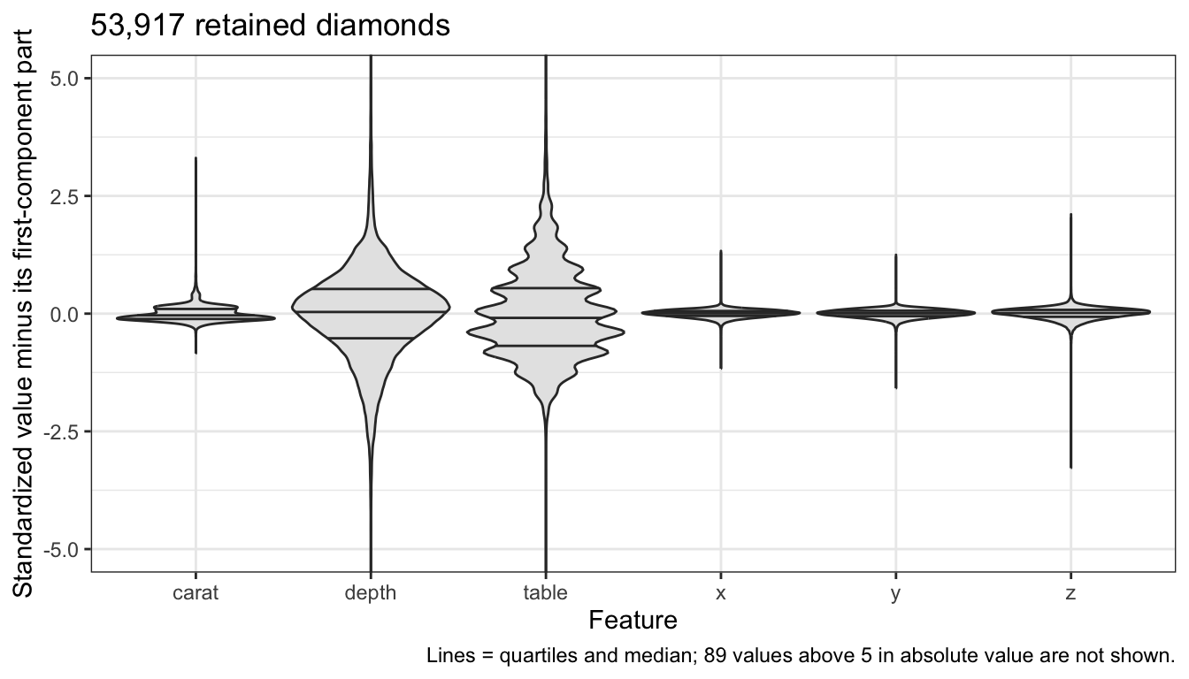

The four size features have almost nothing left: their remaining variances are 0.007 to 0.027. Depth and table keep nearly all of theirs, 1.000 and 0.943. The next direction should be found mostly in depth and table.

23.3.2 Orthogonal directions

The $m$th principal component $Z_m$, with loading vector $\phi_m$ and scores $z_{im} = \tilde x_i\phi_m$, maximizes the sample variance of the scores among unit vectors orthogonal to $\phi_1, \ldots, \phi_{m-1}$, for $m = 2, \ldots, p$.

The eigenvectors of the symmetric matrix $\mathbf{R}$ can be chosen orthonormal. Order them by their eigenvalues $v_1 \ge v_2 \ge \cdots \ge v_p \ge 0$, and assume no ties. Any unit vector is $a = \sum_{m=1}^p c_m\phi_m$ with $\sum_m c_m^2 = 1$, and since $\mathbf{R}\phi_m = v_m\phi_m$,

\[a^\top\mathbf{R}a = \sum_{m=1}^p c_m^2v_m,\]

a weighted average of the eigenvalues. Orthogonality to $\phi_1, \ldots, \phi_{m-1}$ forces $c_1 = \cdots = c_{m-1} = 0$, and the largest weighted average of $v_m, \ldots, v_p$ puts all the weight on $v_m$. So $\phi_m$ is the eigenvector with the $m$th largest eigenvalue, and the scores of the $m$th component have variance $v_m$. All $p$ components come from one eigendecomposition.

Two properties follow.

The scores are uncorrelated. For $m \ne l$, the sample covariance of $z_m$ and $z_l$ is $\frac{1}{n}\phi_m^\top\tilde{\mathbf{X}}^\top\tilde{\mathbf{X}}\phi_l = \phi_m^\top\mathbf{R}\phi_l = v_l\phi_m^\top\phi_l = 0$.
The variances add up to $p$. With $\boldsymbol{\Phi}$ the $p \times p$ matrix whose columns are $\phi_1, \ldots, \phi_p$, which is orthogonal, $\sum_m v_m = \operatorname{tr}\left(\boldsymbol{\Phi}^\top\mathbf{R}\boldsymbol{\Phi}\right) = \operatorname{tr}\left(\mathbf{R}\boldsymbol{\Phi}\boldsymbol{\Phi}^\top\right) = \operatorname{tr}\left(\mathbf{R}\right) = p$, the total variance of the standardized features.

For the diamonds the sum of the six eigenvalues is 6.00, and the largest correlation between two columns of scores is $2.9 \times 10^{-11}$ in absolute value.

23.3.3 prcomp

prcomp() with scale. = TRUE computes the same components.

# Principal components from prcomp().
pca <- prcomp(X, center = TRUE, scale. = TRUE)

# Largest differences from the eigendecomposition, up to sign.
loading_gap <- abs(pca$rotation) - abs(Phi)
loading_diff <- max(abs(loading_gap))
variance_diff <- max(abs(pca$sdev^2 - v))
score_gap <- abs(pca$x) - sqrt((n - 1) / n) * abs(Z)
score_diff <- max(abs(score_gap))

Up to sign, its loadings pca$rotation agree with the eigenvectors of $\mathbf{R}$ to within $1.4 \times 10^{-10}$. prcomp() standardizes with divisor $n - 1$, so its scores pca$x are $\sqrt{(n - 1)/n}$ times the scores here (to within $6.3 \times 10^{-10}$). Its variances pca$sdev^2, computed with divisor $n - 1$ as well, equal the eigenvalues $v_m$ (to within $6.3 \times 10^{-13}$), because the two factors cancel. Its signs are whatever its algorithm returns.

Beyond this course

Singular value decomposition. prcomp() does not form $\mathbf{R}$. It computes the singular value decomposition $\tilde{\mathbf{X}} = \mathbf{U}\mathbf{D}\mathbf{V}^\top$, whose right singular vectors (the columns of $\mathbf{V}$) are the loading vectors and whose squared singular values divided by $n$ are the variances $v_m$; this is more accurate numerically than an eigendecomposition of $\mathbf{R}$.
Best low-dimensional approximation. The closest-line property extends: the first $M$ components span the $M$-dimensional subspace closest to the data in mean squared distance, and $\sum_{m=1}^M z_{im}\phi_m^\top$ is the best rank-$M$ approximation of $\tilde{\mathbf{X}}$.
Variants. Sparse principal components force some loadings to zero, much as the lasso does for coefficient estimates; kernel principal components find nonlinear directions; robust principal components limit the influence of outlying observations.

23.3.4 Variance explained

The proportion of variance explained by component $m$ is

\[\text{PVE}_m = \frac{v_m}{\sum_{l=1}^p v_l} = \frac{v_m}{p},\]

where $v_m$ is the variance of the $m$th component’s scores and the denominator is the total variance of the standardized features. The cumulative PVE of the first $M$ components is $\sum_{m=1}^M\text{PVE}_m$.

Code

# Proportion of variance explained by each component, and cumulatively.
pve <- v / sum(v)
cum_pve <- cumsum(pve)

# Table of the variances and proportions.
pve_tibble <- tibble(Component = paste0("PC", 1:p),
                     `Variance $v_m$` = fmt(v, 3),
                     `PVE` = pct(pve, 2),
                     `Cumulative PVE` = pct(cum_pve, 2))
pve_table <- knitr::kable(pve_tibble, align = "lrrr")

# Scree plot and cumulative PVE, with the 90% level dotted.
scree_types <- c("Component m (scree plot)",
                 "First m components (cumulative)")
type_rep <- rep(scree_types, each = p)
scree_data <- tibble(m = rep(1:p, 2),
                     value = c(pve, cum_pve),
                     type = factor(type_rep, levels = scree_types))
scree_plot <- ggplot(scree_data,
                     aes(x = m,
                         y = value,
                         color = type,
                         shape = type,
                         linetype = type)) +
  geom_hline(yintercept = 0.9, color = "grey50", linetype = "dotted") +
  geom_line() +
  geom_point(size = 2.5) +
  scale_color_manual(values = okabe_ito[c(4, 5)]) +
  scale_x_continuous(breaks = 1:p) +
  scale_y_continuous(labels = scales::label_percent(), limits = c(0, 1)) +
  labs(x = "Component m",
       y = "Proportion of variance explained",
       color = NULL,
       shape = NULL,
       linetype = NULL,
       title = title_all) +
  theme(legend.position = "bottom")

# The component after which the PVE drops by the largest factor.
M_elbow <- which.max(pve[-p] / pve[-1])

# The fewest components whose cumulative PVE reaches 90%.
M_90 <- which(cum_pve >= 0.9)[1]

Component	Variance $v_m$	PVE	Cumulative PVE
PC1	3.999	66.66%	66.66%
PC2	1.284	21.40%	88.06%
PC3	0.683	11.38%	99.44%
PC4	0.031	0.52%	99.95%
PC5	0.002	0.03%	99.98%
PC6	0.001	0.02%	100.00%

The figure plots the PVE of each component, the scree plot, and the cumulative PVE.

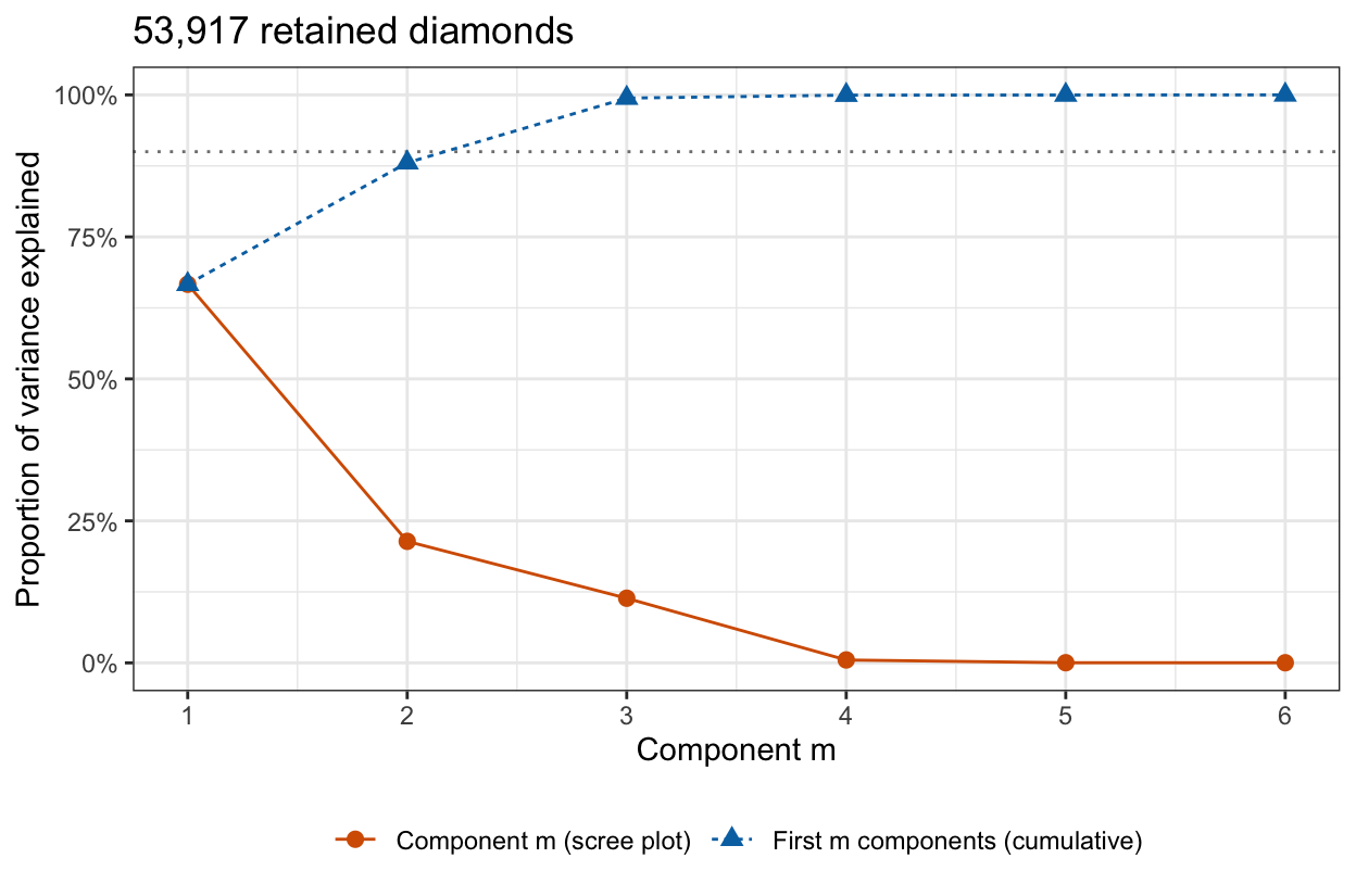
The first component explains 66.7% of the variance of the six features, the second 21.4%, and the third 11.4%. Together the first 3 explain 99.4%, and the last 3 share the remaining 0.56%.

# Component variances from all diamonds, the removed ones included.
cor_all <- cor(diamonds[features])
v_all <- eigen(cor_all, symmetric = TRUE)$values

# The components after the elbow.
small <- (M_elbow + 1):p

# Largest relative change among the other variances, and the ratio of the
# sums of the small ones.
large_change <- max(abs(v_all / v - 1)[-small])
small_ratio <- sum(v_all[small]) / sum(v[small])

Components with small variance are sensitive to a few bad rows. Computed from all 53,940 diamonds, the 23 removed ones included, the first 3 variances change by at most 1.7%, but the last 3 sum to 0.100 instead of 0.034, 3.0 times as much.

23.3.5 Components kept

Keeping the first $M$ components replaces the $p$ features by $M$ new variables, the columns of scores $z_1, \ldots, z_M$; $M$ is the dimension of the reduced feature set. Two common rules choose $M$:

Elbow. Keep the components before the scree plot flattens. Here the PVE falls by a factor of 22 from component 3 to component 4, the largest ratio between consecutive components, so $M = 3$.
Cumulative threshold. Keep the fewest components whose cumulative PVE reaches a chosen level. At 90% (dotted line), $M = 3$; the first 2 reach 88.1%.

Both are judgments: the elbow is read from a picture, and the threshold is a choice. Neither looks at the price. When the components are used to predict a response, the next lecture chooses $M$ by cross-validation instead.

23.4 Scaling

23.4.1 Raw units

The figure shows the six explanatory variables as recorded, each centered at its mean, on one axis.

Code

# Standard deviation of each explanatory variable, in its own unit.
raw_sd <- apply(X, 2, sd_n)
raw_sd_text <- paste0(code(features), " ", fmt(raw_sd, 2))

# Each explanatory variable centered at its mean.
X_centered <- sweep(X, 2, colMeans(X))
unit_labels <- c(carat = "carat (carats)",
                 depth = "depth (%)",
                 table = "table (%)",
                 x = "x (mm)",
                 y = "y (mm)",
                 z = "z (mm)")

# Violins of the centered values, cut at 10 from the mean.
n_cut_raw <- sum(abs(X_centered) > 10)
raw_caption <- paste("Lines = quartiles and median;",
                     n_cut_raw,
                     "values more than 10 from their mean are not shown.")
raw_plot <- as_tibble(X_centered) |>
  pivot_longer(everything(), names_to = "variable") |>
  mutate(variable = factor(unit_labels[variable], levels = unit_labels)) |>
  ggplot(aes(x = variable, y = value)) +
  violin +
  coord_cartesian(ylim = c(-10, 10)) +
  labs(x = "Explanatory variable (unit)",
       y = "Value minus mean, in its own unit",
       title = title_all,
       caption = raw_caption)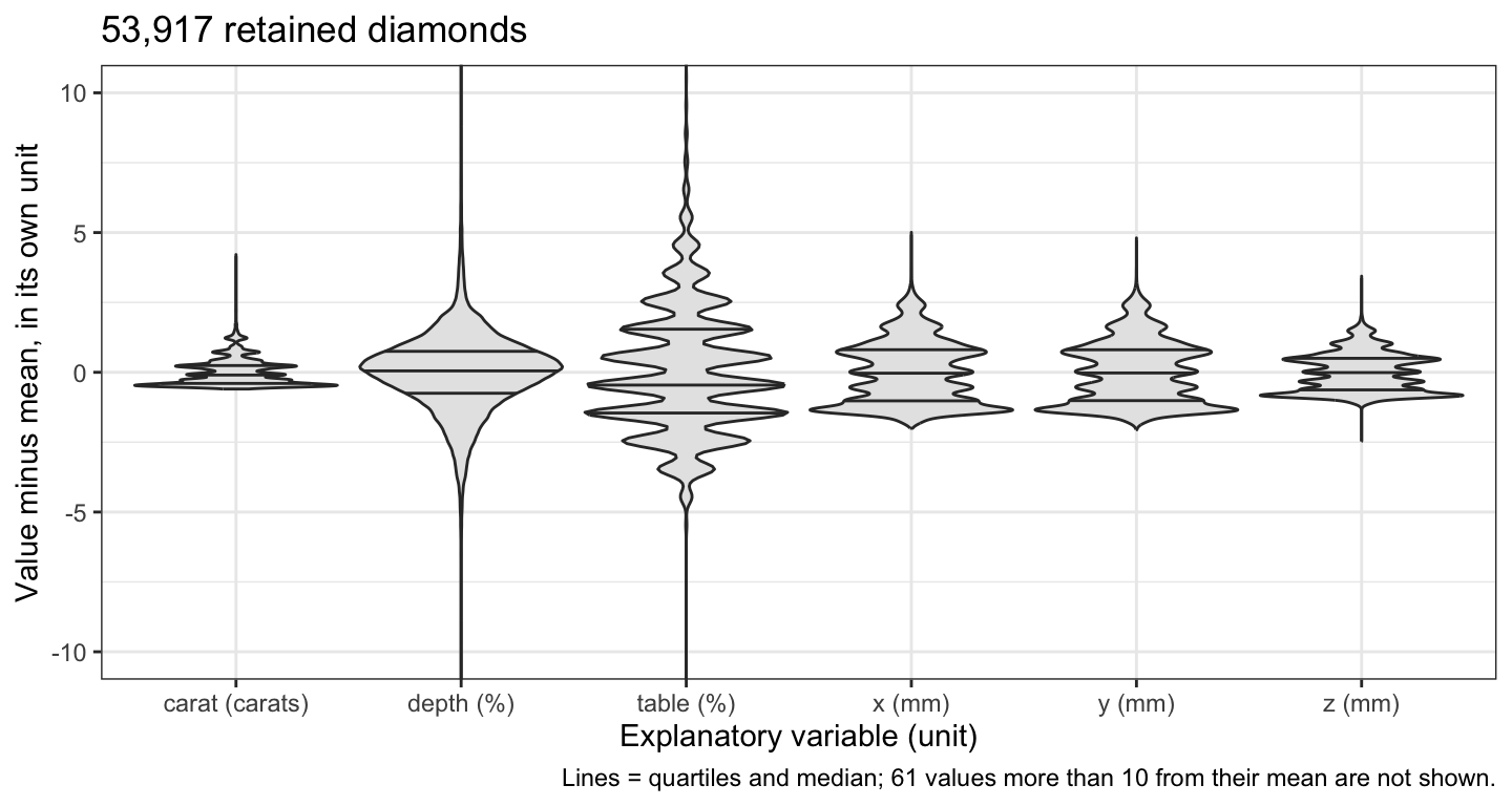

On their own scales the explanatory variables spread very differently: the standard deviations are carat 0.47, depth 1.43, table 2.23, x 1.12, y 1.11, and z 0.69, so table varies most and carat least, in units that cannot be compared.

23.4.2 Unstandardized components

Principal components of the centered but unstandardized explanatory variables maximize $a^\top\mathbf{S}a$, with $\mathbf{S}$ the sample covariance matrix, whose diagonal holds the squared standard deviations above. The figure compares the first loading vector of the standardized features with that of the unstandardized variables, and with that of the unstandardized variables after weight is recorded in milligrams (1 carat = 200 mg) instead of carats.

Code

# First loading vector of a covariance or correlation matrix, signed so its
# largest loading in absolute value is positive.
signed_pc1 <- function(M) {
  phi <- eigen(M, symmetric = TRUE)$vectors[, 1]
  phi * largest_sign(phi)
}

# Explanatory variables with weight in milligrams instead of carats.
X_mg <- X
X_mg[, "carat"] <- 200 * X_mg[, "carat"]
mg_sd <- sd_n(X_mg[, "carat"])

# Covariance matrices, divisor n, in carats and in milligrams.
S <- cov(X) * (n - 1) / n
S_mg <- cov(X_mg) * (n - 1) / n

# Unstandardized first loading vectors and the PVE of their components.
pc1_raw <- signed_pc1(S)
pc1_mg <- signed_pc1(S_mg)
pve_raw <- eigen(S, symmetric = TRUE)$values[1] / sum(diag(S))
pve_mg <- eigen(S_mg, symmetric = TRUE)$values[1] / sum(diag(S_mg))

# Standardized first loading vector in milligrams, and its largest
# difference from the one in carats.
pc1_mg_std <- signed_pc1(cor(X_mg))
pc1_mg_gap <- max(abs(pc1_mg_std - Phi[, 1]))

# Facet labels: each version and the PVE of its first component.
pc1_versions <- c("Standardized",
                  "Unstandardized",
                  "Unstandardized, carat in mg")
pc1_pve <- c(pve[1], pve_raw, pve_mg)
version_labels <- paste0(pc1_versions, "\nPVE ", pct(pc1_pve))

# First loading vector of each version, one facet each.
version_rep <- rep(version_labels, each = p)
feature_rep <- rep(features, 3)
feature_levels <- rev(features)
scaling_data <- tibble(version = factor(version_rep, levels = version_labels),
                       feature = factor(feature_rep, levels = feature_levels),
                       loading = c(Phi[, 1], pc1_raw, pc1_mg))
scaling_plot <- ggplot(scaling_data, aes(x = loading, y = feature)) +
  loading_bars +
  facet_wrap(~ version) +
  labs(x = "Loading on the first component",
       y = NULL,
       title = title_all)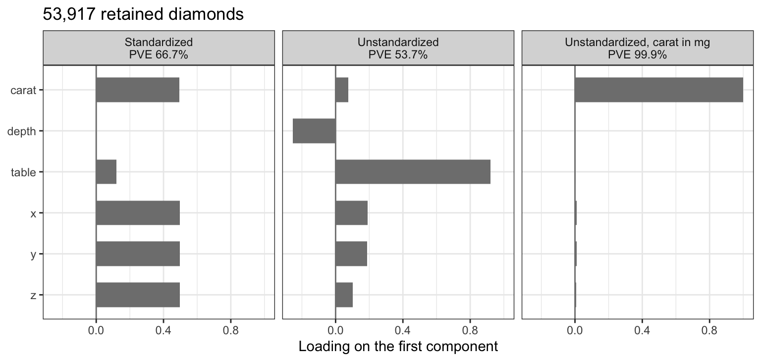

Unstandardized, the first component is mostly table, loading 0.92, the variable with the largest variance, and it no longer measures size. Recording weight in milligrams raises the standard deviation of carat to 94.8 and makes the first component almost entirely weight, loading 1.000, explaining 99.9% of a total variance that weight now dominates.

Standardized features remove the dependence on units: the correlation matrix is the same in carats or milligrams, and the standardized first loading vectors agree to within $1.7 \times 10^{-14}$. The features are therefore standardized before principal component analysis unless the explanatory variables share a unit in which their variances are comparable, as the three dimensions in mm would on their own. Like the means and standard deviations of the ridge and lasso lectures, the loadings are computed from the data, so when components feed a model that is cross-validated, the standardization and the loadings are recomputed from the training folds in each fold.

23.5 Interpretation

23.5.1 Loadings

The figure plots the estimated loadings of all six components.

Code

# Facet label of each component: its name and PVE.
component_labels <- paste0("PC", 1:p, " (PVE ", pct(pve, 2), ")")

# Loadings of all six components, one facet each.
loadings_plot <- as_tibble(Phi, rownames = "feature") |>
  pivot_longer(-feature, names_to = "component", values_to = "loading") |>
  mutate(feature = factor(feature, levels = feature_levels),
         component = str_remove(component, "PC"),
         component = as.integer(component),
         component = factor(component_labels[component],
                            levels = component_labels)) |>
  ggplot(aes(x = loading, y = feature)) +
  loading_bars +
  facet_wrap(~ component, nrow = 2) +
  labs(x = "Loading",
       y = NULL,
       title = title_all)

# First-component loadings of the four size features.
size_load <- Phi[size_vars, 1]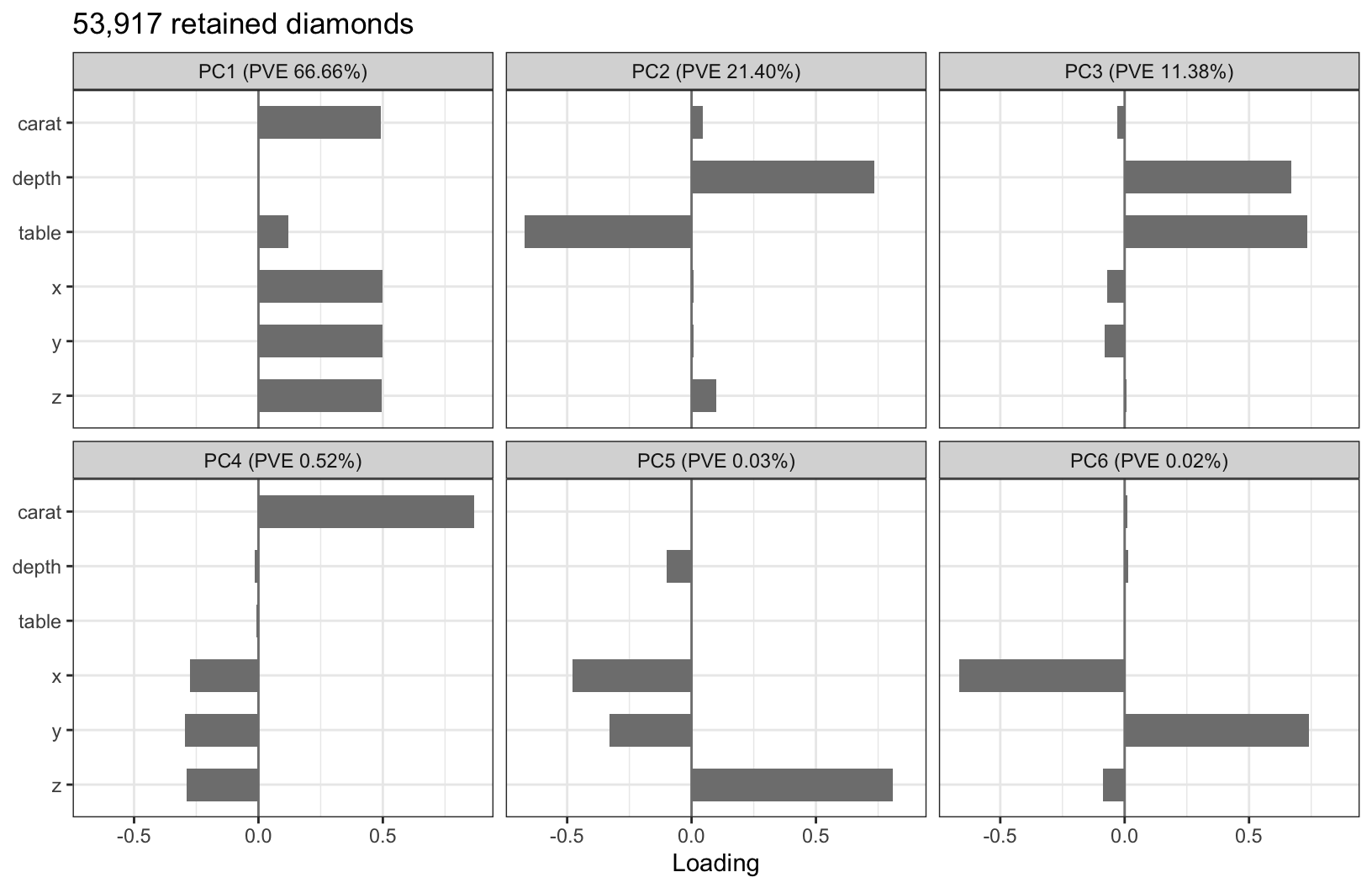

A loading is the weight a feature receives in the component’s score. Each is read relative to the others in its loading vector.

PC1, size. Carat, x, y, and z load 0.49 to 0.50, table 0.12, and depth 0.00. Four perfectly correlated features, uncorrelated with the others, would each load $1/\sqrt 4 = 0.5$. A high score is a large diamond.
PC2, depth against table. Depth loads 0.73 and table −0.67, with the size features near zero. A high score is a deep diamond with a narrow table, a low score a shallow one with a wide table: a contrast in shape, as the two-feature figure found. Depth percentage is z relative to x and y, so the depth part of this component, and of PC3, re-expresses dimensions already in the data rather than adding a measurement.
PC3, depth and table together. Both load positively, 0.67 and 0.73. A high score is a diamond that is both deep and wide-topped.
PC4 to PC6, disagreements among the size measures. These contrast carat, x, y, and z with one another, for example weight against the linear dimensions in PC4, whose carat loading is 0.87. Their variances are small because the four measurements rarely disagree.

23.5.2 Sign

$\phi_m$ and $-\phi_m$ have the same length and give scores with the same variance, $\left(-\phi_m\right)^\top\mathbf{R}\left(-\phi_m\right) = \phi_m^\top\mathbf{R}\phi_m$, so the sign of a loading vector is arbitrary. Flipping it flips every loading and every score of that component and changes no interpretation: “high PC2 is deep and narrow-topped” becomes “low PC2 is deep and narrow-topped.” This chapter flips each vector so that its largest loading in absolute value is positive; prcomp() and other software may return either sign.

23.5.3 Scores

The biplot plots the first two scores of the 1,000 subsampled diamonds, colored by price, and draws the first two loadings of each feature as an arrow.

Code

# First two scores and the price of the subsampled diamonds.
score_data <- tibble(z1 = Z[sub_id, 1],
                     z2 = Z[sub_id, 2],
                     price = kept$price[sub_id])

# Arrows: the first two loadings of each feature, lengthened arrow_scale
# times.
arrow_scale <- 4
arrows <- tibble(feature = features,
                 z1 = arrow_scale * Phi[, 1],
                 z2 = arrow_scale * Phi[, 2])

# The four size arrows nearly coincide; one label marks their common tip.
size_label <- tibble(feature = and_list(size_vars),
                     z1 = max(arrows$z1),
                     z2 = 0)
arrow_labels <- arrows |>
  filter(feature %in% c("depth", "table")) |>
  bind_rows(size_label)

# Scores colored by price, with the loading arrows on top.
biplot_caption <- paste0("Arrows: loadings on PC1 and PC2, times ",
                         arrow_scale,
                         ".")
arrow_head <- arrow(length = unit(0.2, "cm"))
biplot <- ggplot(score_data, aes(x = z1, y = z2)) +
  geom_point(aes(color = price), alpha = 0.7, size = 1.2) +
  scale_color_viridis_c(trans = "log10",
                        labels = scales::label_dollar(accuracy = 1),
                        breaks = c(500, 1000, 3000, 10000)) +
  coord_equal() +
  geom_segment(data = arrows,
               aes(x = 0, y = 0, xend = z1, yend = z2),
               arrow = arrow_head,
               linewidth = 0.7) +
  geom_label(data = arrow_labels,
             aes(label = feature),
             size = 3.2,
             hjust = c(0.5, 0.5, 0),
             nudge_x = c(0, 0, 0.2),
             nudge_y = c(0.3, -0.3, 0)) +
  labs(x = expression("First component score " * z[i1]),
       y = expression("Second component score " * z[i2]),
       color = "Price (log scale)",
       title = title_sub,
       caption = biplot_caption)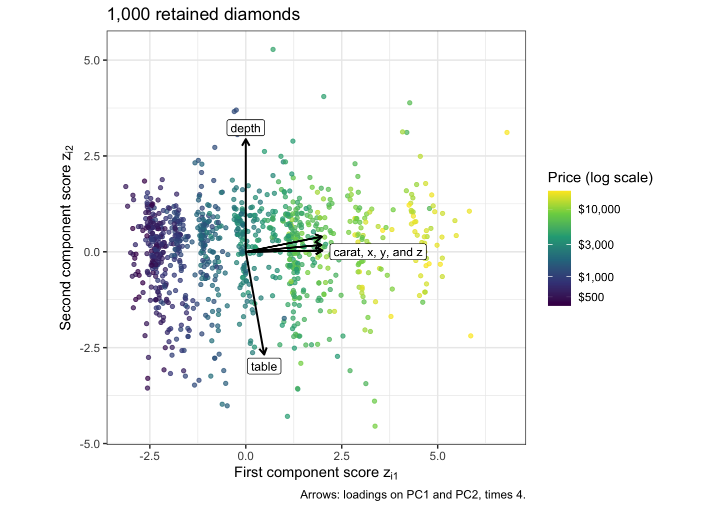

The color changes from left to right, from the cheapest diamonds to the most expensive, and much less from bottom to top. The carat, x, y, and z arrows nearly coincide and point along the first axis; depth points up and table down.

Each row of the $n \times M$ matrix of scores is a diamond described by $M$ new variables in place of its $p$ features. With $M = 2$ the figure is that description.

23.6 Unsupervised learning

23.6.1 Price

Principal component analysis used the six features and never the price. The figure plots price against each component’s scores for the subsampled diamonds; each panel gives the correlation over all $n$ diamonds.

Code

# Correlation of price with each component's scores, and the later
# component with the largest one in absolute value.
price_cor <- drop(cor(kept$price, Z))
top_later <- which.max(abs(price_cor[-1])) + 1

# The smallest loading in absolute value.
smallest_index <- which.min(abs(Phi))
smallest_at <- arrayInd(smallest_index, dim(Phi))
smallest <- list(feature = features[smallest_at[1]],
                 m = smallest_at[2],
                 loading = Phi[smallest_at])

# Price against each component's scores, one facet each.
price_labels <- paste0("PC", 1:p, ": r = ", fmt_math(price_cor))
price_plot <- as_tibble(Z[sub_id, ], .name_repair = ~ price_labels) |>
  mutate(price = kept$price[sub_id]) |>
  pivot_longer(-price, names_to = "component", values_to = "score") |>
  mutate(component = factor(component, levels = price_labels)) |>
  ggplot(aes(x = score, y = price)) +
  geom_point(alpha = 0.3, size = 0.7) +
  facet_wrap(~ component, scales = "free_x", nrow = 2) +
  scale_y_continuous(labels = scales::label_dollar()) +
  labs(x = "Score",
       y = "Price",
       title = title_sub)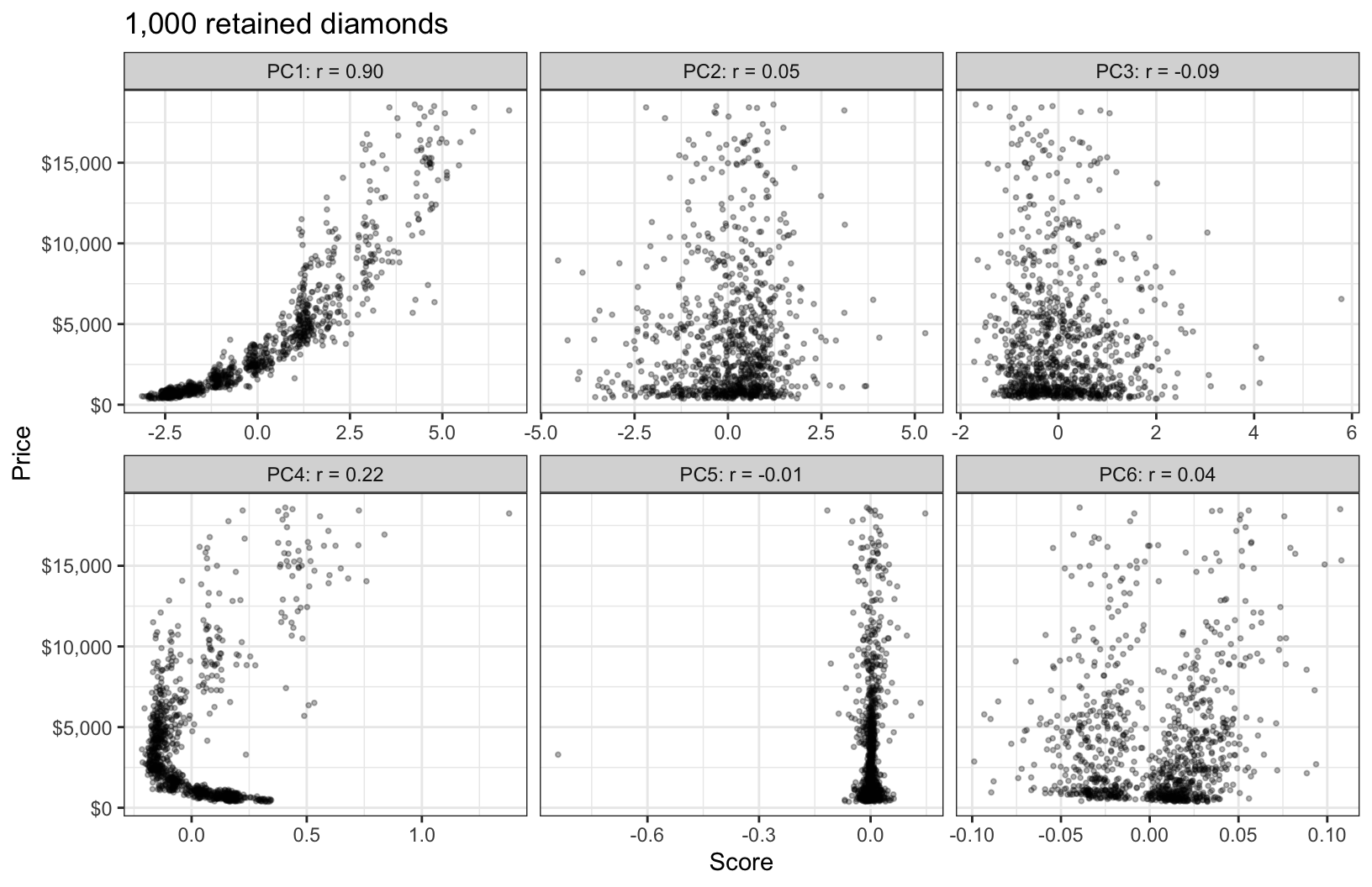

Price rises with the first component’s scores, steeply and with a curve, correlation 0.90. That is an observation about these data, not a fitted model, and nothing in the construction of the first component guaranteed it: the first component is the direction of largest variance among the features; the features of these diamonds happen to vary most in size, and price is also most strongly associated with size. Among the later components the largest correlation in absolute value, 0.22, belongs to PC4, whose scores correlate more strongly with price than those of PC2 (0.05) or PC3 (−0.09), although PC4 explains only 0.52% of the variance while PC2 and PC3 explain 21.4% and 11.4%.

23.6.2 Prediction

Principal component analysis is unsupervised: the loadings, the scores, and the variances are computed from the features alone, and the components are ordered by the variance of the features, not by any relation to a response. The component with the largest variance need not be the most useful for prediction, a component with little variance, such as PC4 here, can carry information about the response that the first few do not, and a rule that keeps the first $M$ components by PVE can discard it.

# Least squares regression of price on all six scores, and its R^2.
price_fit <- lm(kept$price ~ Z)
r2_scores <- summary(price_fit)$r.squared

Because the scores of different components are uncorrelated, the squared correlations of price with the six scores add: they sum to 0.861, which equals the $R^2$ of the least squares regression of price on all six scores, 0.861. Of that total, PC4 accounts for 0.046, and PC2 and PC3 together for 0.010.

Principal components are also not variable selection. Every component is a combination of all $p$ features. Even the smallest loading in absolute value, that of depth on PC1, is $4.6 \times 10^{-5}$, not zero, so computing even the first score of a new diamond requires all six explanatory variables, however few components a model keeps.

23.7 Conclusion

Principal component analysis replaces $p$ correlated features by new variables, the components, ordered by how much of the features’ variance each carries. The features are the standardized explanatory variables. The first component’s loading vector $\phi_1$ is the unit vector that maximizes the sample variance of the scores $z_{i1} = \tilde x_i\phi_1$; a Lagrange multiplier shows that it is the eigenvector of the sample correlation matrix with the largest eigenvalue, and the eigenvalue is the variance of the scores. The same direction minimizes the mean squared distance from the data to a line, because the variance and that distance sum to $p$.

The later components are the remaining eigenvectors, orthogonal directions of decreasing variance. Their scores are uncorrelated, and their variances sum to $p$, so the proportion of variance explained by component $m$ is $v_m/p$. The number of components $M$ kept is the dimension of the reduced feature set; a scree plot’s elbow or a cumulative PVE threshold chooses it by judgment. Components depend on the units of the explanatory variables, so the features are standardized unless the units are comparable. A component is interpreted from its loadings, whose overall sign is arbitrary.

The components are computed without the response. The component with the most variance need not be the best predictor, a low-variance component can matter for prediction, and every component uses every feature.

The next lecture, principal components regression and partial least squares, regresses the log price of the same diamonds on the first $M$ components, chooses $M$ by cross-validation, and compares the components with directions that partial least squares chooses using the response.