# Flea beetles, with the class coded y = 1 (heik) or y = -1 (conc).
beetles <- Sleuth3::ex1613 |>
  mutate(y = if_else(Species == "heik", 1, -1))

count(beetles, Species)
Species n
1 conc 18
2 heik 18After this lecture you should be able to
e1071::svm() fit with a linear kernel and a very large cost, identify the support vectors, and explain why the fitted hyperplane depends only on them,This is the first of three lectures on support vector machines. It covers the maximal margin classifier, a classifier for two classes that cuts the space of the explanatory variables in two with a flat boundary, a hyperplane, chosen to be as far as possible from the observations of both classes. The reading is ISLR2 Section 9.1.
Question. Two species of flea beetle are very similar. Can two measurements of a beetle’s joints separate the species with a straight line, and if so, which line?
Data. Sleuth3::ex1613 records two measurements, in micrometers, of each of 36 beetles from two very similar species of flea beetle (conc and heik); the data come from a 1962 study of discriminant functions in taxonomy by Lubischew. Jnt1 is the measurement of the first joint and Jnt2 of the second. The observations are beetles; each species is a class, and the two explanatory variables are the features.
# Flea beetles, with the class coded y = 1 (heik) or y = -1 (conc).
beetles <- Sleuth3::ex1613 |>
mutate(y = if_else(Species == "heik", 1, -1))
count(beetles, Species) Species n
1 conc 18
2 heik 18# Axes in micrometers, equal scales so that distances and right angles look
# right: Jnt1 every 20, Jnt2 every 10, minor lines midway.
x_scale <- scale_x_continuous(breaks = seq(160, 240, by = 20),
minor_breaks = seq(150, 250, by = 10))
y_scale <- scale_y_continuous(breaks = seq(100, 140, by = 10),
minor_breaks = seq(105, 145, by = 10))
x_limits <- c(155, 245)
y_limits <- c(100, 145)
# The beetles' axes, colored and shaped by species, legend in the empty
# lower-right corner.
beetle_base <- function(x_axis = x_scale, y_axis = y_scale,
xlim = x_limits, ylim = y_limits) {
ggplot(beetles, aes(x = Jnt1, y = Jnt2)) +
x_axis +
y_axis +
coord_fixed(xlim = xlim, ylim = ylim, expand = FALSE) +
scale_color_manual(values = species_colors) +
scale_shape_manual(values = species_shapes) +
labs(x = "First joint, Jnt1 (micrometers)",
y = "Second joint, Jnt2 (micrometers)",
color = "Species", shape = "Species") +
theme(legend.position = "inside",
legend.position.inside = c(0.99, 0.02),
legend.justification = c(1, 0),
legend.direction = "horizontal")
}
# The points on top of any lines drawn before them.
beetle_points <- function(data = beetles) {
geom_point(data = data,
aes(color = Species, shape = Species),
size = 2)
}
beetle_plot <- beetle_base() +
beetle_points()
# Range of each measurement within each species, and the beetles that share
# their measurements with another beetle.
ranges <- beetles |>
group_by(Species) |>
summarize(min1 = min(Jnt1), max1 = max(Jnt1),
min2 = min(Jnt2), max2 = max(Jnt2))
range_of <- function(species, column) {
ranges[[column]][ranges$Species == species]
}
n_shared <- sum(duplicated(beetles[c("Jnt1", "Jnt2")]))
stopifnot(n_shared ==
sum(duplicated(beetles[c("Species", "Jnt1", "Jnt2")])))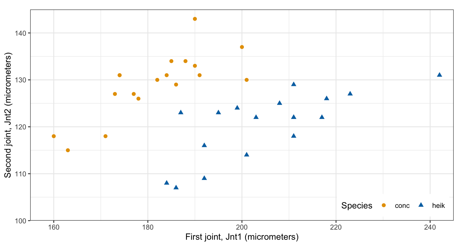
The conc beetles sit up and to the left, with shorter first joints and longer second joints, and the heik beetles down and to the right. Neither measurement alone separates the species: Jnt1 runs from 160 to 201 micrometers in conc and from 184 to 242 in heik. Together they do, with a narrow gap between the two clouds running from lower left to upper right. The measurements are whole micrometers, and 2 pairs of beetles of the same species share both measurements, so 34 distinct points are visible.
The tabs show the beetles and then one line drawn through them, with one side of it shaded.
# A hyperplane beta0 + beta1 x1 + beta2 x2 = 0, drawn as the line
# x2 = -(beta0 + beta1 x1) / beta2, and its two margins at f(x) = -M and
# f(x) = M, dashed.
hyperplane_line <- function(beta, level = 0, linetype = "solid") {
  geom_abline(intercept = (level - beta[1]) / beta[3],
              slope = -beta[2] / beta[3],
              linetype = linetype)
}
margin_lines <- function(beta, M) {
  list(hyperplane_line(beta),
       hyperplane_line(beta, level = -M, linetype = "dashed"),
       hyperplane_line(beta, level = M, linetype = "dashed"))
}

# The example hyperplane -70 + Jnt1 - Jnt2 = 0 and the corners of the
# region where f is positive (below the line, Jnt2 < Jnt1 - 70).
beta_example <- c(-70, 1, -1)
positive_side <- tibble(Jnt1 = c(170, 245, 245, 215),
                        Jnt2 = c(100, 100, 145, 145))

hyperplane_plot <- beetle_base() +
  geom_polygon(data = positive_side, fill = "grey85") +
  hyperplane_line(beta_example) +
  annotate("label", x = 180, y = 138, label = "f(x) < 0") +
  annotate("label", x = 210, y = 108, label = "f(x) > 0") +
  beetle_points()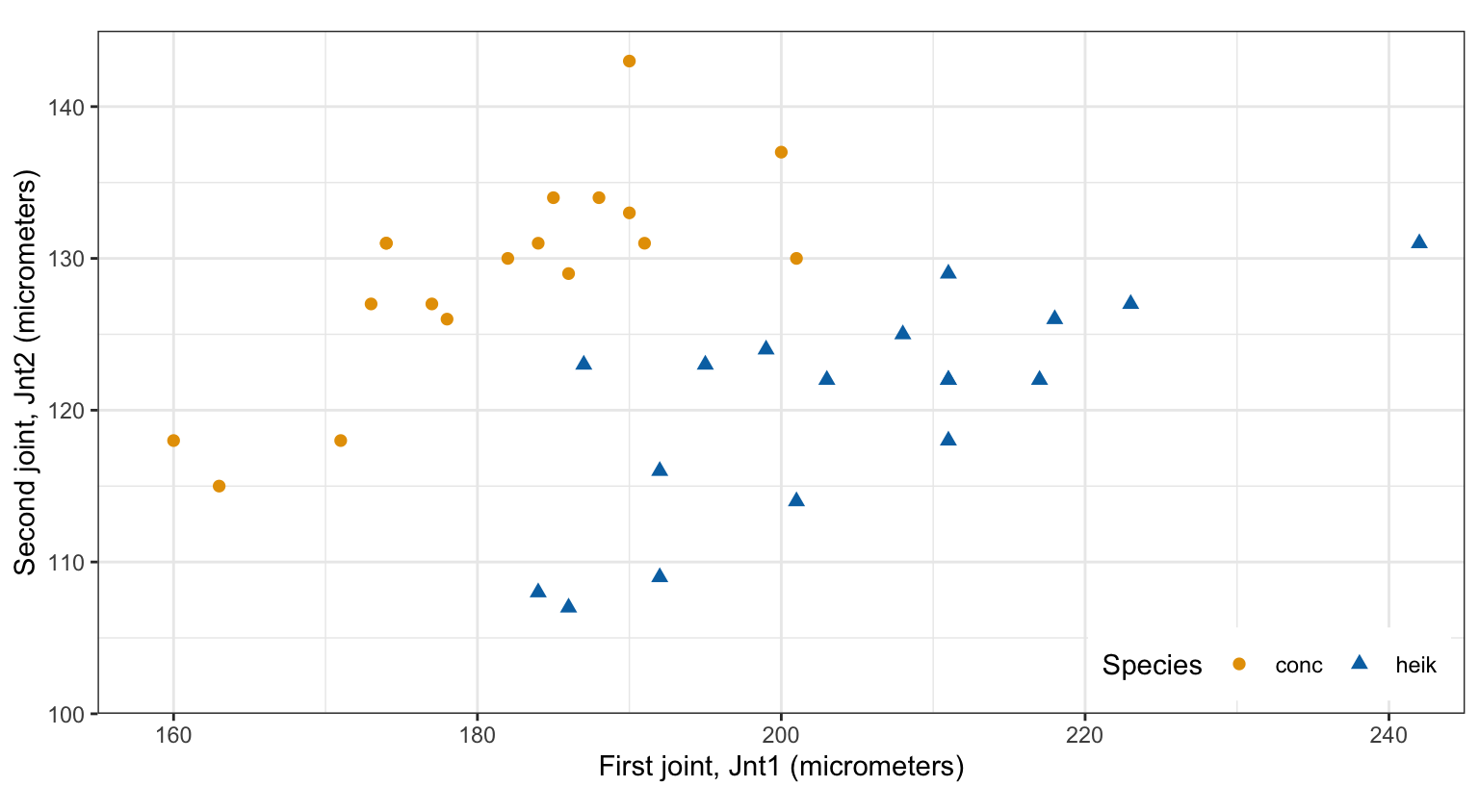
A hyperplane in \(p\) dimensions is the set of points \(X = (X_1, \ldots, X_p)^\top\) that satisfy
\[ \beta_0 + \beta_1 X_1 + \beta_2 X_2 + \cdots + \beta_p X_p = 0, \]
where
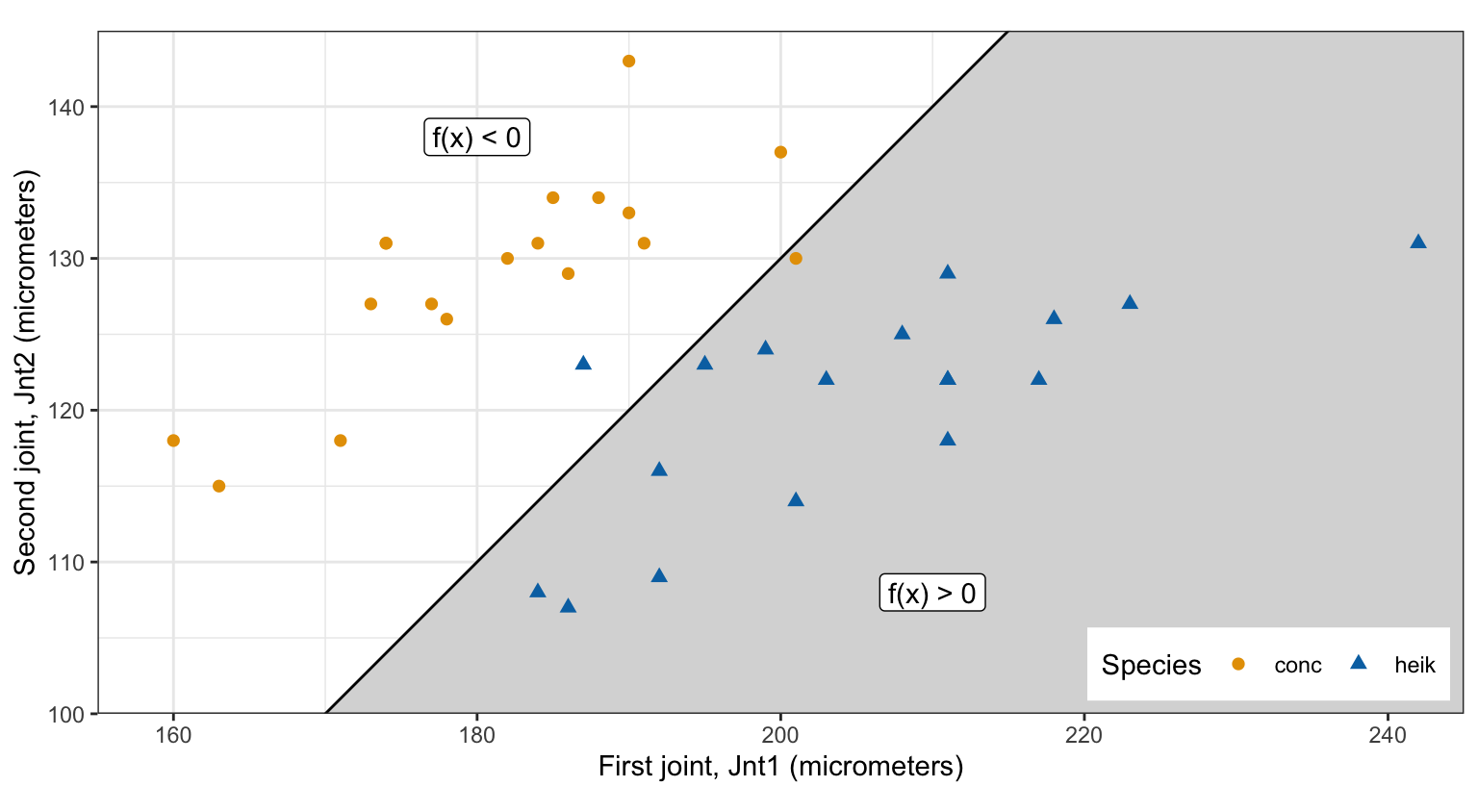
It is a flat affine subspace of dimension \(p - 1\): a point when \(p = 1\), a line when \(p = 2\), a plane when \(p = 3\). With the beetles, \(p = 2\), \(X_1\) is Jnt1, \(X_2\) is Jnt2, and the line in the second tab has \(\beta_0 = -70\), \(\beta_1 = 1\), and \(\beta_2 = -1\).
The normal vector is perpendicular to the hyperplane. If \(x\) and \(x'\) both lie on it, subtracting their equations gives \(\beta^\top\left(x - x'\right) = 0\), so \(\beta\) is orthogonal to every direction within the hyperplane.
For any point \(x = (x_1, \ldots, x_p)^\top\), write
\[ f(x) = \beta_0 + \beta_1 x_1 + \cdots + \beta_p x_p = \beta_0 + \beta^\top x, \]
where \(x_j\) is the \(j\)th coordinate of \(x\). Training observation \(i\), from the next section on, is \(x_i = (x_{i1}, \ldots, x_{ip})^\top\) with \(j\)th coordinate \(x_{ij}\): a single subscript \(j\) on a generic point \(x\) names a coordinate, and a single subscript \(i\) names an observation.
The hyperplane is the set where \(f(x) = 0\). It divides the space in two: \(f(x) > 0\) on one side, the side \(\beta\) points toward, and \(f(x) < 0\) on the other. In the second tab, \(f\) is positive in the shaded region below the line, where Jnt1 exceeds Jnt2 by more than 70 micrometers, and negative above it. Beetles of both species lie on both sides of this line.
Let \(x_0\) be the point of the hyperplane closest to \(x\). Then \(x - x_0\) is perpendicular to the hyperplane, so \(x - x_0 = t\,\beta/\|\beta\|\) for some number \(t\), where \(\|\beta\| = \left(\sum_{j=1}^p \beta_j^2\right)^{1/2}\) and \(|t|\) is the distance from \(x\) to the hyperplane. Because \(f(x_0) = 0\),
\[ f(x) = f(x) - f(x_0) = \beta^\top\left(x - x_0\right) = t\,\frac{\beta^\top\beta}{\|\beta\|} = t\,\|\beta\|, \]
so
\[ t = \frac{f(x)}{\|\beta\|} = \frac{\beta_0 + \beta^\top x}{\|\beta\|}, \]
where \(t\), whose sign gives the side, is the signed distance from \(x\) to the hyperplane.
Multiplying \(\beta_0\) and \(\beta\) by the same nonzero number leaves the hyperplane unchanged, so they can always be scaled to \(\|\beta\|^2 = \sum_{j=1}^p \beta_j^2 = 1\). With this unit normal vector, \(t = f(x)\): \(f(x)\) itself is the signed distance.
Beetle 1, a conc beetle, has Jnt1 \(= 191\) and Jnt2 \(= 131\), so for the line in the second tab \(f(x) = -70 + 191 - 131 =
-10\). The normal vector \((1, -1)^\top\) has length \(\sqrt{2}\), so beetle 1 lies \(7.07\) micrometers from the line, on the negative side. Dividing all three numbers by \(\sqrt{2}\) gives the same line with a unit normal vector, \(-49.50 +
0.71X_1 -
0.71X_2 = 0\), for which \(f(x) = -7.07\) is the signed distance directly.
The tabs show the beetles and then three lines drawn through them, each named in the legend by the angle of its normal vector, defined below.
# Matrix of the two features, one row per beetle.
x_mat <- as.matrix(beetles[c("Jnt1", "Jnt2")])
is_heik <- beetles$y == 1

# For a unit normal vector at angle theta (degrees), the gap between the
# smallest beta'x among heik and the largest among conc, and the beta0 that
# puts the hyperplane midway.
unit_normal <- function(theta) {
  c(cos(theta * pi / 180), sin(theta * pi / 180))
}
gap_of <- function(theta) {
  projection <- drop(x_mat %*% unit_normal(theta))
  min(projection[is_heik]) - max(projection[!is_heik])
}
midway_beta <- function(theta) {
  projection <- drop(x_mat %*% unit_normal(theta))
  beta0 <- -(min(projection[is_heik]) + max(projection[!is_heik])) / 2
  c(beta0, unit_normal(theta))
}

# The angles (to 0.001 degree) at which the beetles are separable.
separable_theta <- range(Filter(function(theta) gap_of(theta) > 0,
                                seq(-90, 90, by = 0.001)))

# Three separating hyperplanes, at three angles of the normal vector, each
# with its own line type, named in a legend by the angle in degrees (with a
# typographic minus sign).
theta_sep <- c(-70, -66, -64)
stopifnot(all(sapply(theta_sep, gap_of) > 0))
angle_label <- function(theta) {
  paste0(sub("^-", "\u2212", theta), "\u00b0")
}
sep_lines <- tibble(theta = theta_sep) |>
  mutate(beta = lapply(theta, midway_beta),
         intercept = sapply(beta, function(b) -b[1] / b[3]),
         slope = sapply(beta, function(b) -b[2] / b[3]),
         label = factor(angle_label(theta), angle_label(theta)))
sep_linetypes <- setNames(c("solid", "longdash", "dotted"),
                          levels(sep_lines$label))

# Both legends stacked in the empty lower-right corner.
separating_plot <- beetle_base() +
  geom_abline(data = sep_lines,
              aes(intercept = intercept, slope = slope, linetype = label)) +
  scale_linetype_manual(values = sep_linetypes) +
  beetle_points() +
  labs(linetype = "Normal vector angle") +
  theme(legend.box = "vertical",
        legend.box.just = "right",
        legend.key.width = unit(1.2, "cm"))

# Check: each of the three puts every beetle on its own class's side.
y_f <- sapply(theta_sep, function(theta) {
  beta <- midway_beta(theta)
  beetles$y * drop(beta[1] + x_mat %*% beta[-1])
})
stopifnot(all(y_f > 0))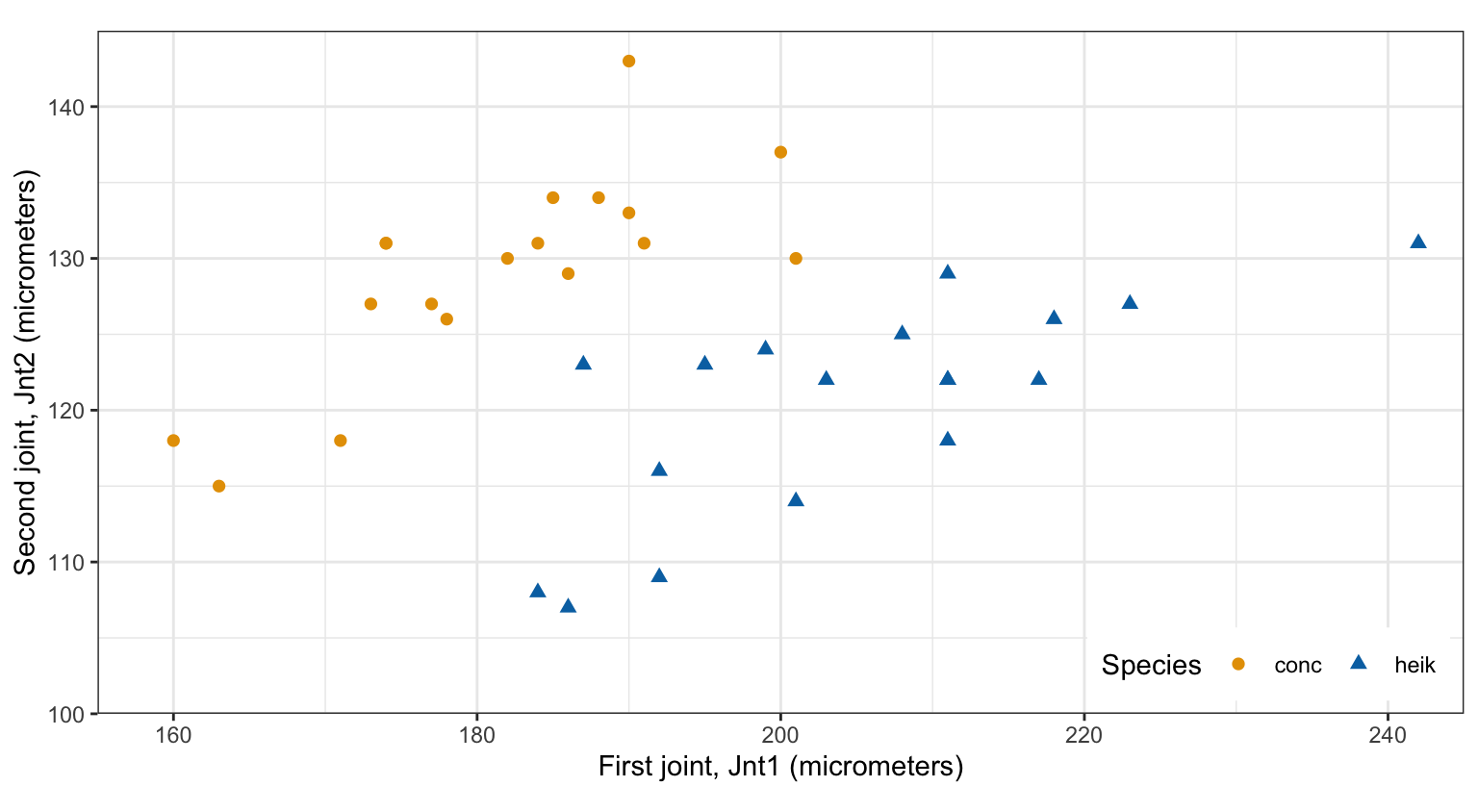
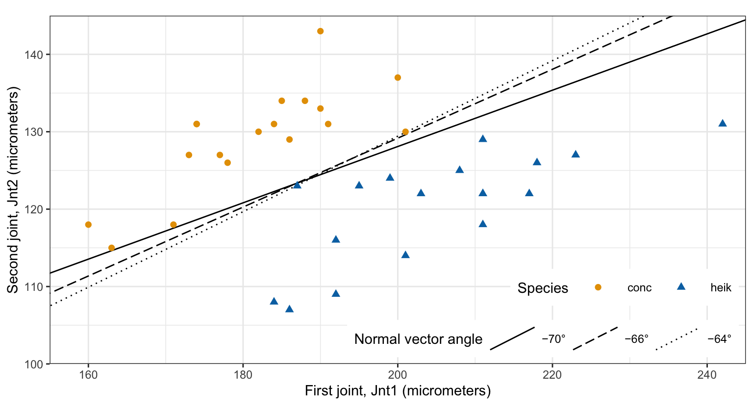
Each of the three lines has every heik beetle on one side and every conc beetle on the other.
For two classes, code the class of observation \(i\) as
\[ y_i = \begin{cases} 1 & \text{if observation } i \text{ is in the first class,}\\ -1 & \text{if observation } i \text{ is in the second class,}\end{cases} \]
where \(i = 1, \ldots, n\) indexes the \(n\) training observations, with features \(x_i = (x_{i1}, \ldots, x_{ip})^\top\). This coding is for the geometry, not a response for regression: the sign of \(y_i\) says which side of the hyperplane observation \(i\) belongs on. Which class gets \(1\) is arbitrary. For the beetles, \(y_i = 1\) for heik and \(y_i = -1\) for conc (the column y above), \(n = 36\), and \(p = 2\).
A hyperplane separates the classes when every observation with \(y_i = 1\) has \(f(x_i) > 0\) and every observation with \(y_i = -1\) has \(f(x_i) < 0\). With the \(\pm 1\) coding the two conditions are one,
\[ y_i\left(\beta_0 + \beta_1 x_{i1} + \cdots + \beta_p x_{ip}\right) > 0 \quad \text{for all } i = 1, \ldots, n. \]
The classes are separable when some hyperplane satisfies this. A separating hyperplane gives a classifier: assign a point \(x\) to the class of the sign of \(f(x)\).
When the classes are separable, a separating hyperplane can be shifted a little, or rotated a little, and still separate them, because each strict inequality \(y_i f(x_i) > 0\) still holds after a small enough change in \(\beta_0, \ldots, \beta_p\). So there are infinitely many separating hyperplanes. The three lines in the second tab have normal vectors at angles −70, −66, and −64 degrees from the Jnt1 axis; every angle between −71.6 and −63.4 degrees gives some separating line through the gap. A classifier needs a rule for picking one.
The tabs show the middle line of the three, the one at −66 degrees, and then the same line with dashed lines parallel to it through the beetles closest to it.
# The middle separating hyperplane, its margin (smallest distance from a
# beetle), and the beetles at that distance.
theta_one <- theta_sep[2]
beta_one <- midway_beta(theta_one)
distance_one <- beetles$y * drop(beta_one[1] + x_mat %*% beta_one[-1])
M_one <- min(distance_one)
closest_one <- beetles[distance_one - M_one < 1e-8, ]

one_line_plot <- beetle_base() +
  hyperplane_line(beta_one) +
  beetle_points()

margin_one_plot <- beetle_base() +
  margin_lines(beta_one, M_one) +
  geom_point(data = closest_one, shape = 1, size = 5) +
  beetle_points()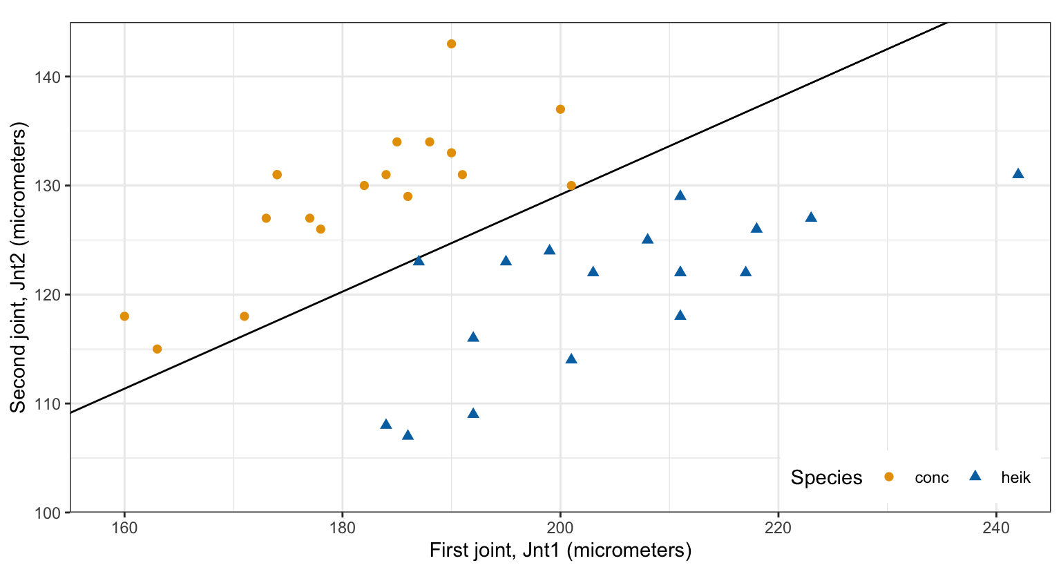
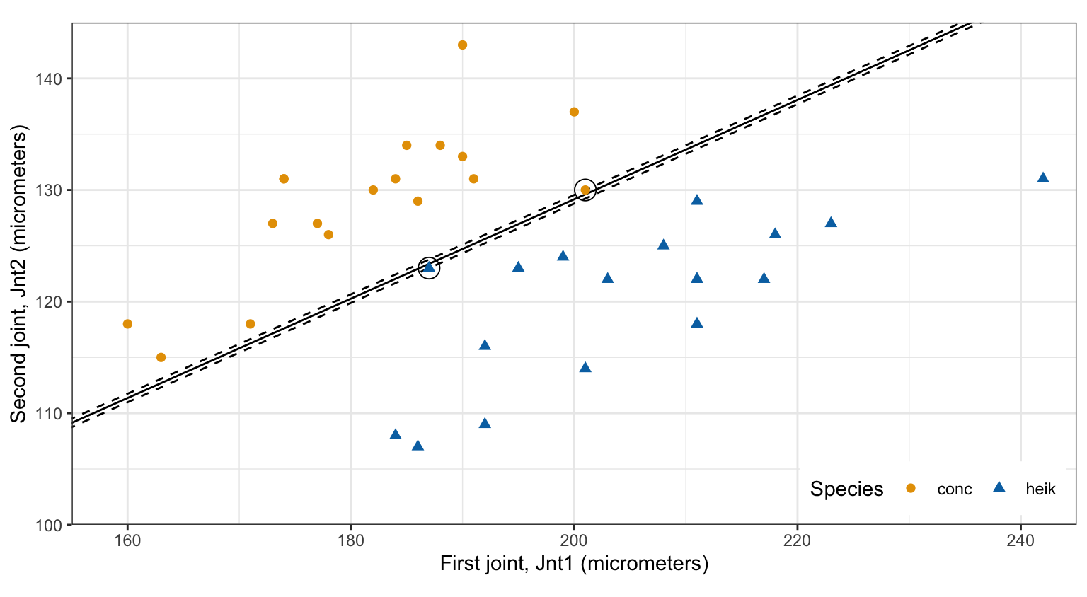
The margin of a separating hyperplane is the smallest distance from it to any training observation. With a unit normal vector, \(y_i f(x_i)\) is the distance from \(x_i\) to the hyperplane (positive, since the hyperplane separates), so the margin is \(\min_i y_i f(x_i)\). The line in the tabs, with normal vector at −66 degrees, has a margin of 0.35 micrometers, set by the circled beetles (13 and 35); no beetle lies between the dashed lines.
The maximal margin hyperplane is the separating hyperplane with the largest margin, and the maximal margin classifier classifies by the side of it a point is on. It is the separating hyperplane farthest from the training observations of both classes, so it has the most room for a new observation to fall near the training observations of its class and still be classified correctly.
The maximal margin hyperplane solves
\[ \begin{aligned} \underset{\beta_0, \beta_1, \ldots, \beta_p, M}{\text{maximize}} \quad & M \\ \text{subject to} \quad & \sum_{j=1}^p \beta_j^2 = 1, \\ & y_i\left(\beta_0 + \beta_1 x_{i1} + \cdots + \beta_p x_{ip}\right) \ge M \quad \text{for all } i = 1, \ldots, n, \end{aligned} \]
where \(M\) is the margin. The pieces:
Fix the unit normal vector \(\beta\) and ask which \(\beta_0\) is best. The constraints split by class:
\[ \beta_0 + \beta^\top x_i \ge M \text{ when } y_i = 1, \qquad -\beta_0 - \beta^\top x_i \ge M \text{ when } y_i = -1. \]
Both hold for all \(i\) exactly when \(M \le \beta_0 + \min_{i: y_i = 1}\beta^\top x_i\) and \(M \le -\beta_0 - \max_{i: y_i = -1}\beta^\top x_i\). Adding the two inequalities removes \(\beta_0\):
\[ 2M \le \Delta(\beta) = \min_{i: y_i = 1}\beta^\top x_i - \max_{i: y_i = -1}\beta^\top x_i, \]
where \(\Delta(\beta)\) is the gap between the classes along \(\beta\): the distance, measured along \(\beta\), between the closest observations of the two classes. Equality holds when the two bounds are equal, at
\[ \beta_0 = -\frac{1}{2}\left(\min_{i: y_i = 1}\beta^\top x_i + \max_{i: y_i = -1}\beta^\top x_i\right). \]
So for a given normal vector, the best hyperplane sits midway between the classes and its margin is \(\Delta(\beta)/2\). The classes are separable along \(\beta\) exactly when \(\Delta(\beta) > 0\). The three lines above were placed this way.
What remains is to choose the direction of \(\beta\) to make the gap largest. With \(p = 2\), a unit normal vector is \(\beta = (\cos\theta, \sin\theta)^\top\) for an angle \(\theta\), so the search is over one number. The figure plots the margin \(\Delta(\beta)/2\) of the midway hyperplane against \(\theta\), for every angle at which the beetles are separable.
# Margin of the midway hyperplane on a fine grid of angles of the normal
# vector, where the beetles are separable.
direction_grid <- tibble(theta = seq(-72, -63, by = 0.001)) |>
  mutate(margin = sapply(theta, gap_of) / 2) |>
  filter(margin > 0)
best_direction <- slice_max(direction_grid, margin, with_ties = FALSE)

# The three separating hyperplanes of the earlier figure.
sep_points <- tibble(theta = theta_sep,
                     margin = sapply(theta_sep, gap_of) / 2)

direction_plot <- ggplot(direction_grid, aes(x = theta, y = margin)) +
  geom_line() +
  geom_point(data = sep_points, size = 2) +
  geom_label(data = sep_points, aes(label = angle_label(theta)),
             nudge_y = 0.06, size = 3.5) +
  geom_point(data = best_direction, shape = 1, size = 4) +
  scale_x_continuous(breaks = seq(-72, -64, by = 2),
                     minor_breaks = seq(-71, -63, by = 2)) +
  scale_y_continuous(breaks = seq(0, 0.6, by = 0.2),
                     minor_breaks = seq(0.1, 0.7, by = 0.2)) +
  coord_cartesian(xlim = c(-72, -63), ylim = c(0, 0.7), expand = FALSE) +
  labs(x = expression("Angle of the normal vector, " * theta * " (degrees)"),
       y = "Margin (micrometers)")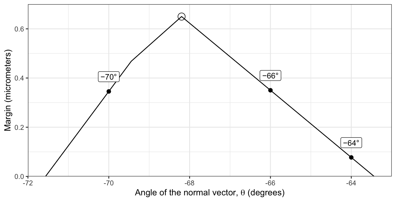
The margin rises to a single peak, circled, at \(\theta = -68.2\) degrees, with margin 0.65 micrometers; the three labeled points are the three lines of the earlier figure, at −70, −66, and −64 degrees. With more features the direction cannot be searched on a grid, and the problem is solved as a quadratic program, which e1071::svm() does.
e1071::svm() with kernel = "linear" fits a hyperplane in the features. In e1071, cost is a penalty on observations that fall inside the margin or on the wrong side of the hyperplane; a very large cost forbids them, so on separable data the fit is the maximal margin hyperplane. The next lecture explains cost. scale = FALSE keeps both features in micrometers, so the margin is a distance in micrometers; svm() by default standardizes each feature, which changes the distances and so changes which hyperplane has the largest margin. tolerance tightens the solver’s stopping rule (its default is 1e-3) so the estimates are accurate to more digits than are printed.
# Maximal margin classifier: linear kernel, a very large cost.
mmc_fit <- svm(Species ~ Jnt1 + Jnt2, data = beetles,
               kernel = "linear", cost = 1e5, scale = FALSE,
               tolerance = 1e-8)
mmc_fit
Call:
svm(formula = Species ~ Jnt1 + Jnt2, data = beetles, kernel = "linear",
    cost = 1e+05, tolerance = 1e-08, scale = FALSE)


Parameters:
   SVM-Type:  C-classification
 SVM-Kernel:  linear
       cost:  1e+05

Number of Support Vectors:  3
The printout gives the settings and the number of support vectors, defined below.
svm() does not report \(\hat\beta_0, \ldots, \hat\beta_p\) directly. It solves the same problem in a rescaled form. Dividing the unit-norm \(\beta_0\) and \(\beta\) by \(M\), write \(w_0 = \beta_0/M\) and \(w = \beta/M\); then \(\|w\| = 1/M\), and the constraints become \(y_i\left(w_0 + w^\top x_i\right) \ge 1\). Maximizing \(M\) is the same as minimizing \(\|w\|\) subject to these constraints, which is the form svm() solves. Undoing the rescaling gives
\[ \hat\beta_0 = \frac{\hat w_0}{\|\hat w\|}, \qquad \hat\beta = \frac{\hat w}{\|\hat w\|}, \qquad \hat M = \frac{1}{\|\hat w\|}. \]
Here \(\hat w_0\) and \(\hat w\) are the versions with heik, coded \(y = 1\), on the positive side. svm() works in its own sign, in which its decision values are positive for the class of the first training observation, here conc, which is why the chapter checks the sign in code: it stores the weighted sum of the support vectors (the rows of SV, with weights coefs), which is \(-\hat w\), and rho, which is \(\hat w_0\).
# w and w0 with heik on the positive side (svm() makes the class of the
# first beetle, conc, positive).
w <- -drop(t(mmc_fit$coefs) %*% mmc_fit$SV)
w0 <- mmc_fit$rho

# Unit-norm estimates and the margin.
norm_w <- sqrt(sum(w^2))
beta_hat <- c(beta0 = w0, w) / norm_w
M_hat <- 1 / norm_w
round(c(beta_hat, M = M_hat), 4)
beta0 Jnt1 Jnt2 M
45.4025 0.3714 -0.9285 0.6499 # Fitted values: with a unit normal vector, the signed distance from each
# beetle to the fitted hyperplane.
f_hat <- function(data) {
drop(beta_hat["beta0"] +
as.matrix(data[c("Jnt1", "Jnt2")]) %*% beta_hat[c("Jnt1", "Jnt2")])
}
f_beetles <- f_hat(beetles)
distance_beetles <- beetles$y * f_beetles
# The sign convention: svm()'s decision values are positive for the class
# of the first training beetle, conc, so they are -(w0 + w'x).
decision <- attr(predict(mmc_fit, beetles, decision.values = TRUE),
"decision.values")
stopifnot(colnames(decision) == "conc/heik",
isTRUE(all.equal(drop(decision), -norm_w * f_beetles,
check.attributes = FALSE)))
# The prose reads beta1 as positive (toward heik) and beta2 as negative.
stopifnot(beta_hat["Jnt1"] > 0, beta_hat["Jnt2"] < 0)
# Unit norm, and every beetle at distance at least M_hat on its own side.
stopifnot(abs(sum(beta_hat[-1]^2) - 1) < 1e-12,
min(distance_beetles) > M_hat - 1e-6)
# No weight at the cost bound: no beetle violates the margin.
stopifnot(max(abs(mmc_fit$coefs)) < mmc_fit$cost / 100)
# A cost 100 times larger gives the same hyperplane and margin.
larger_fit <- svm(Species ~ Jnt1 + Jnt2, data = beetles,
kernel = "linear", cost = 1e7, scale = FALSE,
tolerance = 1e-8)
w_larger <- -drop(t(larger_fit$coefs) %*% larger_fit$SV)
beta_larger <- c(larger_fit$rho, w_larger) / sqrt(sum(w_larger^2))
stopifnot(max(abs(beta_larger - beta_hat)) < 1e-6)
# The measurements are whole micrometers, and the margin is less than one.
resolution <- 1
stopifnot(all(c(beetles$Jnt1, beetles$Jnt2) %% resolution == 0),
M_hat < resolution)
# The grid search over angles finds the same margin and direction.
theta_hat <- atan2(beta_hat["Jnt2"], beta_hat["Jnt1"]) * 180 / pi
stopifnot(abs(best_direction$margin - M_hat) < 1e-3,
abs(best_direction$theta - theta_hat) < 0.01)\(\hat\beta_0\) is in micrometers, and \(\hat\beta_1\) and \(\hat\beta_2\) are micrometers of distance per micrometer of a feature. \(\hat\beta_0 =
45.40\) is \(\hat f\) at the origin, a beetle with both joints of length 0: the origin lies 45.40 micrometers from the hyperplane on the heik side, far outside the data. \(\hat\beta_1 =
0.37\): one more micrometer of first joint increases the beetle’s signed distance, \(\hat f\), by 0.37 micrometers. \(\hat\beta_2 = -0.93\): one more micrometer of second joint decreases it by 0.93 micrometers. \(\hat\beta_1^2 + \hat\beta_2^2 = 1\), and the normal vector’s angle, −68.2 degrees, and the margin \(\hat M =
0.65\) micrometers are those of the peak of the grid search. Refitting with a cost 100 times larger gives the same estimates to six decimal places.
The fitted values \(\hat f(x_i) = \hat\beta_0 + \hat\beta_1 x_{i1} + \hat\beta_2 x_{i2}\) are the signed distances of the beetles from the hyperplane. The figure shows the maximal margin hyperplane (solid), the margins at \(\hat f(x) = \pm\hat M\) (dashed), and the beetles on the margins circled; the second tab zooms in on the gap.
# Support vectors, the rows of the data svm() kept.
support <- beetles[mmc_fit$index, ]

# The maximal margin hyperplane, margins, and circled support vectors.
mmc_layers <- function(beta, M, support_data) {
  list(margin_lines(beta, M),
       geom_point(data = support_data, shape = 1, size = 5))
}
mmc_plot <- beetle_base() +
  mmc_layers(beta_hat, M_hat, support) +
  beetle_points()

# The same, zoomed in on the gap: every 5 micrometers, minor lines every 1,
# the resolution of the measurements, so each beetle sits on a grid crossing.
zoom_x <- scale_x_continuous(breaks = seq(170, 205, by = 5),
                             minor_breaks = seq(170, 205, by = 1))
zoom_y <- scale_y_continuous(breaks = seq(115, 135, by = 5),
                             minor_breaks = seq(115, 135, by = 1))
mmc_zoom_plot <- beetle_base(zoom_x, zoom_y,
                             xlim = c(170, 205), ylim = c(115, 135)) +
  mmc_layers(beta_hat, M_hat, support) +
  beetle_points() +
  theme(legend.position = "none")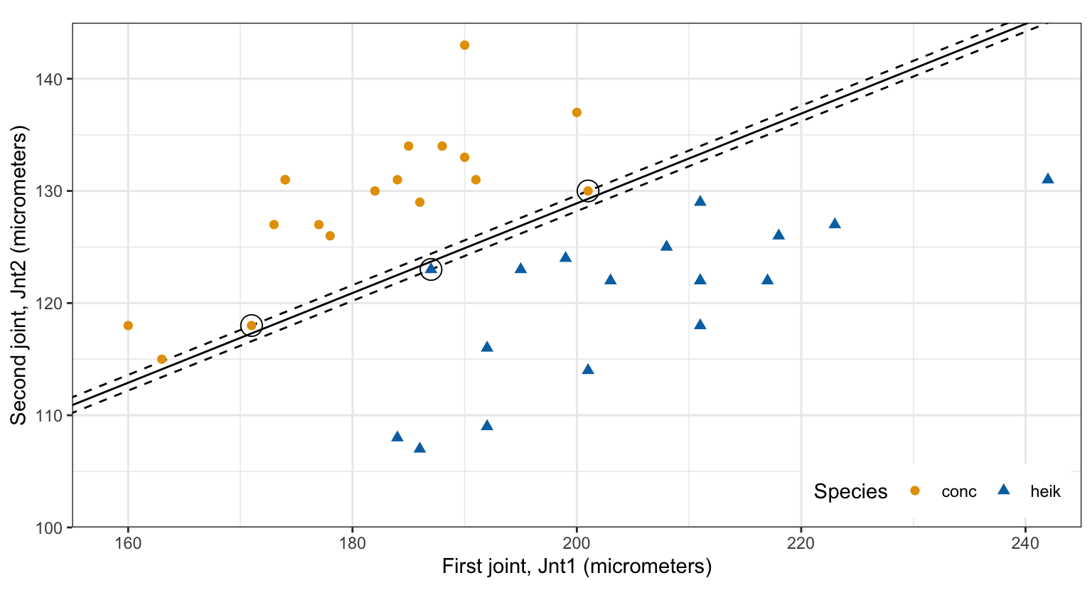
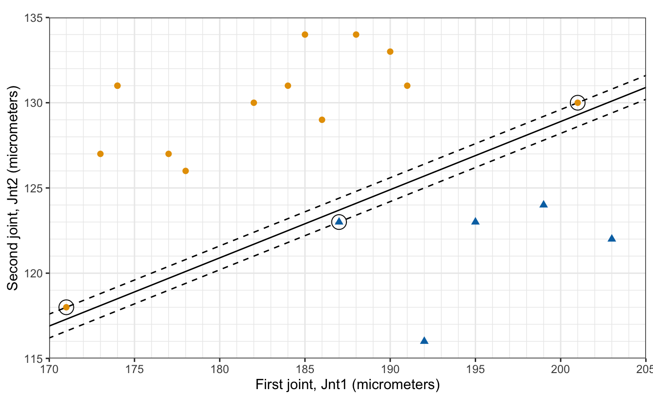
The margin is 0.65 micrometers, less than the 1-micrometer resolution of the measurements: the species are separable, but only just.
The figure is the maximal margin hyperplane of the beetles again; this section is about the circled beetles.
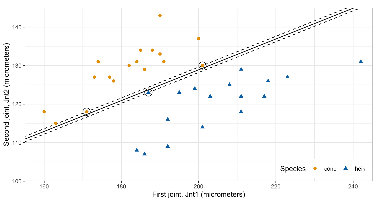
The support vectors are the training observations on the margin, those with \(y_i \hat f(x_i) = \hat M\). They are vectors in \(p\)-dimensional space, and they support the hyperplane in the sense that if any of them moved, the hyperplane would move. For the beetles they are 3 beetles, 5 (conc), 13 (conc), and 35 (heik).
# Signed distance of each beetle, and its distance on its own side.
x_beetles <- as.matrix(beetles[c("Jnt1", "Jnt2")])
beetles <- beetles |>
  mutate(f_hat = drop(beta_hat["beta0"] + x_beetles %*% beta_hat[-1]),
         distance = y * f_hat)

# Beetles on the margin: distance M_hat, up to the solver's accuracy.
beetles |>
  filter(distance - M_hat < 1e-6) |>
  select(Specimen, Species, Jnt1, Jnt2, f_hat)
Specimen Species Jnt1 Jnt2 f_hat
1 5 conc 171 118 -0.6499337
2 13 conc 201 130 -0.6499337
3 35 heik 187 123 0.6499337# The beetles at distance M_hat are the rows svm() kept as support vectors.
on_margin <- beetles$Specimen[beetles$distance - M_hat < 1e-6]
stopifnot(setequal(on_margin, support$Specimen))
# The support vectors of each species.
conc_support <- filter(support, Species == "conc")
heik_support <- filter(support, Species == "heik")
stopifnot(nrow(conc_support) == 2, nrow(heik_support) == 1)The two conc support vectors lie on the dashed line on the conc side and the one heik support vector on the other: the margin cannot grow without one of them crossing it.
The fitted hyperplane depends on the training data only through the support vectors. The constraint \(y_i\left(\beta_0 + \beta^\top x_i\right) \ge M\) of any other observation holds with room to spare at the solution, so deleting it, or moving it anywhere that keeps it outside the margin, leaves the solution unchanged. Deleting a support vector removes a constraint that was holding the margin down, and the solution changes. The table refits the maximal margin classifier to four sets of beetles.
# Fit the maximal margin classifier to some beetles and return its unit-norm
# estimates, margin, and support vectors.
fit_mmc <- function(data) {
  fit <- svm(Species ~ Jnt1 + Jnt2, data = data,
             kernel = "linear", cost = 1e5, scale = FALSE,
             tolerance = 1e-8)
  w <- -drop(t(fit$coefs) %*% fit$SV)
  norm_w <- sqrt(sum(w^2))
  list(beta = c(beta0 = fit$rho, w) / norm_w,
       M = 1 / norm_w,
       support = data$Specimen[fit$index])
}

# A beetle that is not a support vector: the one farthest from the
# hyperplane. A support vector to delete: the conc one with the longer
# first joint.
far_beetle <- beetles$Specimen[which.max(beetles$distance)]
deleted_support <- conc_support$Specimen[which.max(conc_support$Jnt1)]

# The four sets of beetles, named, and the fit to each.
refit_names <- c("All beetles",
                 paste("Without beetle", far_beetle),
                 "Support vectors only",
                 paste("Without beetle", deleted_support))
refit_data <- list(beetles,
                   filter(beetles, Specimen != far_beetle),
                   filter(beetles, Specimen %in% support$Specimen),
                   filter(beetles, Specimen != deleted_support))
refits <- setNames(lapply(refit_data, fit_mmc), refit_names)

refit_table <- tibble(
  Beetles = names(refits),
  n = c(nrow(beetles), nrow(beetles) - 1, nrow(support), nrow(beetles) - 1),
  beta0 = sapply(refits, function(r) r$beta["beta0"]),
  beta1 = sapply(refits, function(r) r$beta["Jnt1"]),
  beta2 = sapply(refits, function(r) r$beta["Jnt2"]),
  M = sapply(refits, function(r) r$M),
  support = sapply(refits, function(r) paste(sort(r$support),
                                             collapse = ", "))
) |>
  knitr::kable(digits = 4,
               col.names = c("Beetles", "$n$", "$\\hat\\beta_0$",
                             "$\\hat\\beta_1$", "$\\hat\\beta_2$",
                             "$\\hat M$", "Support vectors"),
               align = "lcrrrrl")

# The first three agree to six decimal places; the fourth does not.
same_as_all <- function(r) {
  max(abs(c(r$beta, r$M) - c(beta_hat, M_hat)))
}
stopifnot(sapply(refits[1:3], same_as_all) < 1e-6,
          same_as_all(refits[[4]]) > 0.1)

# The deleted support vector, refit without it: its fitted value.
refit_sv <- refits[[4]]
deleted_x <- beetles |>
  filter(Specimen == deleted_support) |>
  select(Jnt1, Jnt2) |>
  unlist()
f_deleted <- refit_sv$beta["beta0"] + sum(refit_sv$beta[-1] * deleted_x)
theta_sv <- atan2(refit_sv$beta["Jnt2"], refit_sv$beta["Jnt1"]) * 180 / pi

# The prose says the refit puts the deleted conc beetle on the heik side.
stopifnot(f_deleted > 0)| Beetles | \(n\) | \(\hat\beta_0\) | \(\hat\beta_1\) | \(\hat\beta_2\) | \(\hat M\) | Support vectors |
|---|---|---|---|---|---|---|
| All beetles | 36 | 45.4025 | 0.3714 | -0.9285 | 0.6499 | 5, 13, 35 |
| Without beetle 11 | 35 | 45.4025 | 0.3714 | -0.9285 | 0.6499 | 5, 13, 35 |
| Support vectors only | 3 | 45.4025 | 0.3714 | -0.9285 | 0.6499 | 5, 13, 35 |
| Without beetle 13 | 35 | 3.4795 | 0.5450 | -0.8384 | 2.2638 | 1, 5, 35 |
Deleting beetle 11, the beetle farthest from the hyperplane, or deleting all 33 beetles that are not support vectors, gives the same estimates and margin to the four decimal places shown (and to six). Deleting beetle 13, a support vector, changes the normal vector’s angle from −68.2 to −57.0 degrees and the margin from 0.65 to 2.26 micrometers.
The figure adds two beetles that are not in the data, A and B, marked by crosses, to the maximal margin hyperplane of the training beetles.
# Two new beetles, their fitted values (signed distances), and the class of
# the sign.
new_beetles <- tibble(Beetle = c("A", "B"),
                      Jnt1 = c(190, 230),
                      Jnt2 = c(125, 120))
new_beetles <- new_beetles |>
  mutate(f_hat = f_hat(new_beetles),
         class = if_else(f_hat > 0, "heik", "conc"))
f_new <- setNames(new_beetles$f_hat, new_beetles$Beetle)

# The prose says A is inside the margin and B well outside it.
stopifnot(abs(f_new["A"]) < M_hat, f_new["B"] > 10 * M_hat)

new_plot <- beetle_base() +
  mmc_layers(beta_hat, M_hat, support) +
  beetle_points() +
  geom_point(data = new_beetles, shape = 4, size = 3, stroke = 1.2) +
  geom_label(data = new_beetles, aes(label = Beetle),
             nudge_x = 4, nudge_y = 3)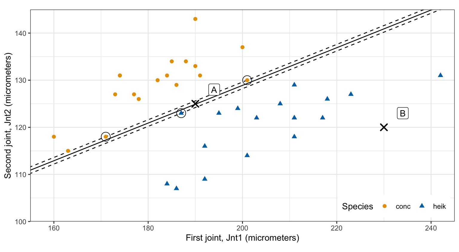
A has Jnt1 \(= 190\) and Jnt2 \(=
125\), in the gap between the species; B has Jnt1 \(= 230\) and Jnt2 \(= 120\), among the heik beetles.
A new observation \(x^* = (x^*_1, \ldots, x^*_p)^\top\) is classified by the sign of
\[ \hat f(x^*) = \hat\beta_0 + \hat\beta_1 x^*_1 + \cdots + \hat\beta_p x^*_p, \]
to the class coded \(y = 1\) if \(\hat f(x^*) > 0\) and to the class coded \(y = -1\) if \(\hat f(x^*) < 0\). For the beetles,
conc;heik.predict() returns the same classes:
# Predicted species of the two new beetles.
predict(mmc_fit, new_beetles)
1 2
conc heik
Levels: conc heikBecause \(\hat\beta\) has unit length, \(\left|\hat f(x^*)\right|\) is the distance from \(x^*\) to the hyperplane in micrometers. The training observations of each class lie on its side, at least \(\hat M\) from the hyperplane. A new observation far from it keeps its class under any small tilt or shift of the hyperplane; one near it does not. So the larger \(\left|\hat f(x^*)\right|\), the more confident the classification. B lies 19.41 micrometers from the hyperplane, well into the heik side. A lies 0.09 micrometers from it, less than the margin of 0.65, inside the gap where no training beetle lies: a slight tilt or shift of the hyperplane would change its class. The distance ranks confidence but is not a probability.
The figure shows each beetle’s first joint alone, by species, with the range of first joints shared by the two species shaded. Points are jittered vertically.
# The range of Jnt1 in which beetles of both species lie, and the beetles in
# it.
overlap <- c(range_of("heik", "min1"), range_of("conc", "max1"))
n_overlap <- sum(between(beetles$Jnt1, overlap[1], overlap[2]))

# The same for Jnt2.
overlap2 <- c(range_of("conc", "min2"), range_of("heik", "max2"))

strip_plot <- ggplot(beetles,
                     aes(x = Jnt1, y = Species,
                         color = Species, shape = Species)) +
  annotate("rect", xmin = overlap[1], xmax = overlap[2],
           ymin = -Inf, ymax = Inf, fill = "grey85") +
  geom_jitter(width = 0, height = 0.15, size = 2) +
  scale_color_manual(values = species_colors) +
  scale_shape_manual(values = species_shapes) +
  x_scale +
  coord_cartesian(xlim = x_limits, ylim = c(0.6, 2.4), expand = FALSE) +
  labs(x = "First joint, Jnt1 (micrometers)", y = NULL) +
  theme(legend.position = "none")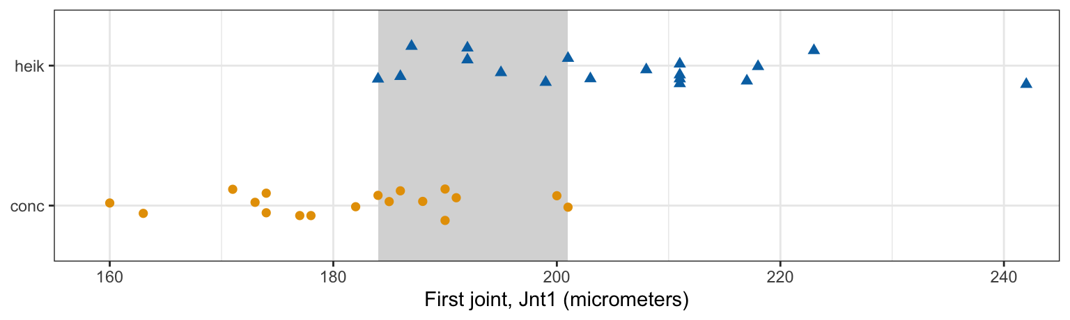
With \(p = 1\) a hyperplane is a single point, a cut point on the Jnt1 axis, and it separates the species only if every conc beetle lies below it and every heik beetle above it, or the reverse. The largest conc first joint, 201, exceeds the smallest heik one, 184, and 17 beetles lie in the shaded range between them. No cut point separates the species, so the constraints \(y_i\left(\beta_0 + \beta_1 x_{i1}\right) \ge M\) cannot all hold with \(M > 0\), and no maximal margin hyperplane exists. The same is true of Jnt2 alone, whose ranges overlap from 115 to 131 micrometers.
The beetles are separable with both measurements, but in many classification problems the classes overlap whatever features are used. There the maximal margin classifier has no solution.
The tabs show the fit to all beetles, the fit without support vector 13 (its position marked by a cross), and the fit with one added conc beetle that is not in the data (boxed).
# Without the deleted support vector, which is marked by a cross.
deleted_beetle <- filter(beetles, Specimen == deleted_support)
without_beetles <- filter(beetles, Specimen != deleted_support)
without_plot <- beetle_base() +
  mmc_layers(refit_sv$beta, refit_sv$M,
             filter(beetles, Specimen %in% refit_sv$support)) +
  beetle_points(without_beetles) +
  geom_point(data = deleted_beetle, shape = 4, size = 3, stroke = 1.2)

# With one added conc beetle in the gap, on the heik side of the original
# hyperplane.
added_beetle <- tibble(Specimen = 99,
                       Species = factor("conc", levels(beetles$Species)),
                       Jnt1 = 184,
                       Jnt2 = 122,
                       y = -1)
added_beetles <- bind_rows(select(beetles, Specimen, Species, Jnt1, Jnt2, y),
                           added_beetle)
refit_added <- fit_mmc(added_beetles)
added_plot <- beetle_base() +
  mmc_layers(refit_added$beta, refit_added$M,
             filter(added_beetles, Specimen %in% refit_added$support)) +
  beetle_points(added_beetles) +
  geom_point(data = added_beetle, shape = 0, size = 5)

# The original hyperplane puts the added beetle on the heik side; the refit
# still separates all the beetles, with the added one a support vector.
f_added <- f_hat(added_beetle)
added_x <- as.matrix(added_beetles[c("Jnt1", "Jnt2")])
added_distance <- added_beetles$y *
  drop(refit_added$beta["beta0"] + added_x %*% refit_added$beta[-1])
stopifnot(f_added > 0,
          all(added_distance > 0),
          99 %in% refit_added$support)
theta_added <- atan2(refit_added$beta["Jnt2"],
                     refit_added$beta["Jnt1"]) * 180 / pi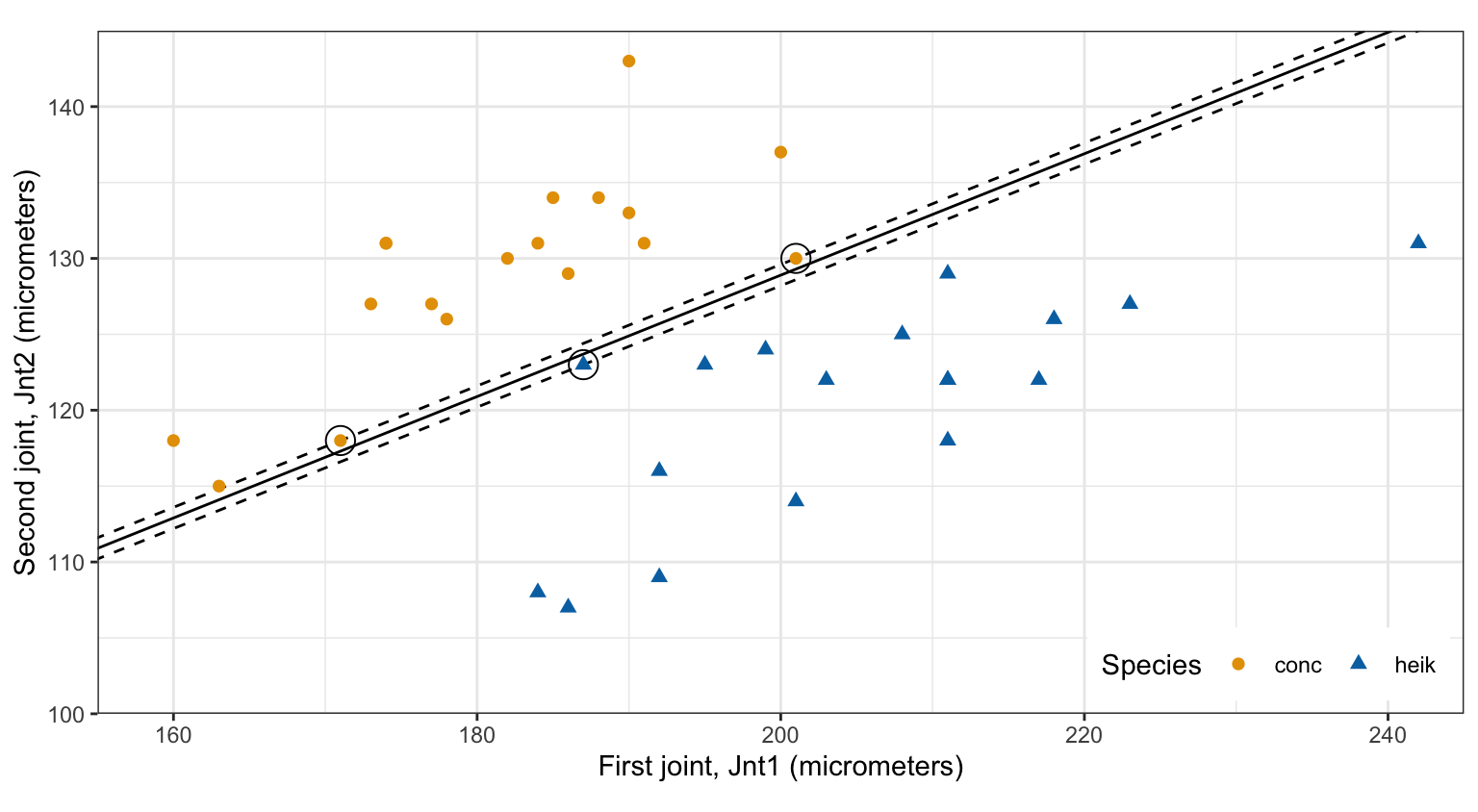
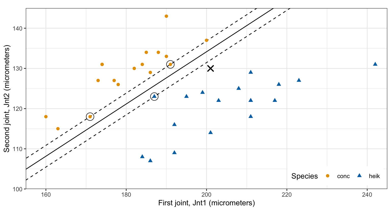
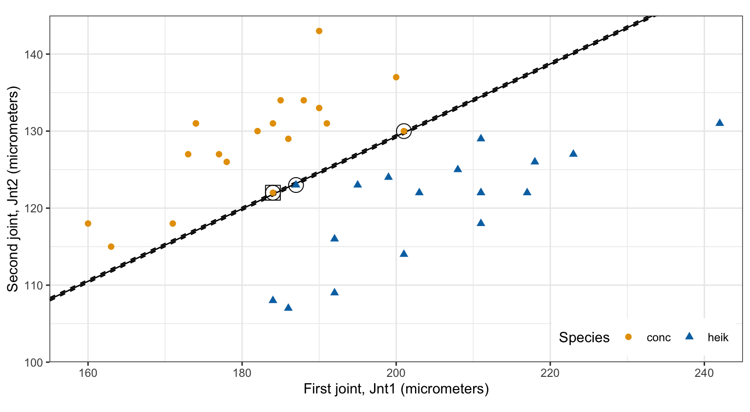
Without beetle 13, the hyperplane tilts to an angle of −57.0 degrees, the margin grows from 0.65 to 2.26 micrometers, and beetle 13 itself, a conc beetle, has fitted value 4.02: the refit puts it on the heik side. The added conc beetle, at Jnt1 \(= 184\) and Jnt2 \(= 122\) (boxed), lies in the gap, 0.46 micrometers on the heik side of the original hyperplane. The beetles are still separable with it, and refitting tilts the hyperplane to −64.8 degrees, puts the added beetle on the margin, and shrinks the margin to 0.19 micrometers. The maximal margin hyperplane is set by a few observations, the support vectors, so a change in one observation near the boundary can move it far. A classifier that moves this much with one observation has high variance, and fitting the training observations perfectly can overfit them.
The rescaled problem in the Estimates section, minimizing \(\|w\|^2/2\) subject to \(y_i\left(w_0 + w^\top x_i\right) \ge 1\), is the hard-margin support vector machine. It is a convex quadratic program, and its Lagrangian dual is a quadratic program in one multiplier \(\alpha_i \ge 0\) per observation, whose solution gives \(\hat w = \sum_i \alpha_i y_i x_i\) with \(\alpha_i > 0\) only for the support vectors (the Karush-Kuhn-Tucker conditions). That is why svm() stores \(\hat w\) as a weighted sum of the support vectors: its coefs are the products \(\alpha_i y_i\), in its own sign. The dual depends on the data only through the inner products \(x_i^\top x_{i'}\), which is what lets kernels replace them. See The Elements of Statistical Learning (Hastie, Tibshirani, and Friedman), Section 4.5.2, or Computer Age Statistical Inference, Section 19.1.
A hyperplane in \(p\) dimensions is the set where \(f(x) = \beta_0 + \beta^\top x = 0\). The normal vector \(\beta\) is perpendicular to it, the sign of \(f(x)\) says which side \(x\) is on, and when \(\sum_j \beta_j^2 = 1\), \(f(x)\) is the signed distance from \(x\) to it.
Coding two classes as \(y_i = \pm 1\) makes \(y_i f(x_i) > 0\) the condition for a hyperplane to separate them. Separable classes have infinitely many separating hyperplanes. The maximal margin hyperplane is the one with the largest margin, the smallest distance to a training observation. It solves the problem of maximizing \(M\) subject to \(\sum_j \beta_j^2 = 1\) and \(y_i\left(\beta_0 + \beta^\top x_i\right) \ge M\); for a fixed normal vector the best hyperplane is midway between the classes, with margin half the gap between them. e1071::svm() with a linear kernel, scale = FALSE for features in common units, and a very large cost fits it, and the estimates and the margin are recovered from its coefs, SV, and rho.
The support vectors are the observations on the margin, and the fitted hyperplane depends only on them. A new observation is classified by the sign of \(\hat f(x^*)\), and \(\left|\hat f(x^*)\right|\) measures confidence as a distance. The classifier has two limitations: when the classes overlap no separating hyperplane exists, and when they do not, moving, deleting, or adding one observation near the boundary can move the hyperplane far.
The next lecture covers the support vector classifier, which allows some observations to fall inside the margin or on the wrong side of the hyperplane, so that it exists for overlapping classes and depends less on any single observation.