# The 100 absorbance columns.
channels <- sprintf("x_%03d", 1:100)
p <- length(channels)

# Rows that repeat an earlier row in every column, and the distinct meats.
meats_all <- modeldata::meats
n_duplicates <- sum(duplicated(meats_all))
meats <- distinct(meats_all)
n_meats <- nrow(meats)25 High Dimensions
TipLearning objectives
After this lecture you should be able to
- explain why, when the model matrix \(\mathbf{X}\) has more columns than rows, \(\mathbf{X}^\top\mathbf{X}\) is singular, the least squares estimate is not unique, and a least squares fit can have training RSS 0 and training \(R^2 = 1\),
- interpret the training \(R^2\), the training MSE, the overall \(F\)-test, and \(\hat\sigma\) of a least squares fit with \(d\) close to \(n\), and explain why none of them estimates the test MSE,
- explain why \(C_p\), AIC, and BIC cannot choose a model size when \(p \ge n - 1\): with \(\sigma^2\) fixed at the estimate from the model with all \(p\) features, that estimate is \(0/0\), and taking it to be 0 reduces \(C_p\) and BIC to the training MSE; with \(\sigma^2\) estimated in each model, as
AIC()andBIC()do, both go to \(-\infty\) at a perfect fit, - choose \(\lambda\) or \(M\) for ridge regression, the lasso, PCR, and PLS by \(k\)-fold cross-validation on the training data, with the standardization and the PCR and PLS directions recomputed inside each fold, and compare the chosen fits with the null model by test MSE, and
- explain why, when the features are highly correlated, the set of features the lasso selects changes from fold to fold within a training sample and is not the set of features that matters.
Every earlier lecture in this chapter had more training observations than features, so least squares had a unique fit, and the other methods traded a little bias for less variance. This lecture’s data have more features than training observations, \(p > n\), the high-dimensional setting, where least squares fails outright and the choice of flexibility decides whether a fit predicts at all.
25.1 Meat spectra
25.1.1 Data
Question. From a small training sample, how well can the fat content of chopped meat be predicted from how much near-infrared light it absorbs at each of more wavelengths than there are training observations?
Data. modeldata::meats was recorded on a Tecator Infratec food analyzer. Each row is one meat, a sample of finely chopped meat; these notes call the observations meats, after the data set, and keep the word “sample” for a set of observations, as in “training sample.” The analyzer shines near-infrared light, at wavelengths from 850 to 1050 nm, just beyond visible red, through the meat and records its absorbance at 100 channels spread over that range: absorbance is \(-\log_{10}\) of the fraction of the light that passes through, so an absorbance of 2 means 1% passes through. Water, fat, and protein absorb these wavelengths differently, so the spectrum carries information about the composition. The fat content, fat, in percent, was measured separately by chemical analysis, which is slow; predicting it from the spectrum, which the analyzer records quickly, is the practical goal. The columns x_001, …, x_100 are the absorbances, in order of wavelength.
NoteCode
Of the 215 rows, 22 repeat an earlier row in all 103 columns. A test meat identical to a training meat is not new data, and a fit that passes through every training meat would predict it exactly, so the repeats are removed, leaving 193 meats. The test meats are split off before any plotting or fitting.
# The training sample size.
n_train <- 50

# Training meats: a random sample; every other meat is a test meat.
train_id <- sample(n_meats, n_train)
train <- meats[train_id, ]
test <- meats[-train_id, ]
n_test <- nrow(test)

# Folds for 10-fold cross-validation of the training meats.
n_folds <- 10
fold_labels <- rep(seq_len(n_folds), length.out = n_train)
fold_id <- sample(fold_labels)

# Absorbances and fat of the training and test meats.
X_train <- as.matrix(train[channels])
X_test <- as.matrix(test[channels])
y_train <- train$fat
y_test <- test$fat

# Number of training meats whose spectra are plotted below.
n_show <- 6
That leaves a training sample of 50 meats and 143 test meats. The figure plots the spectra of 6 training meats, chosen to span the range of fat content.
NoteCode
# Training meats evenly spaced in rank of fat content.
ranks <- round(seq(1, n_train, length.out = n_show))
shown <- order(y_train)[ranks]

# One row per shown meat and channel.
spectra <- as_tibble(X_train[shown, ]) |>
  mutate(fat = y_train[shown], meat = factor(seq_len(n_show))) |>
  pivot_longer(all_of(channels),
               names_to = "channel",
               values_to = "absorbance") |>
  mutate(channel = as.integer(sub("x_", "", channel)))

# Heights for labels at y, moved up where needed so that consecutive labels
# are at least gap apart.
spread_labels <- function(y, gap) {
  sorted <- order(y)
  height <- y[sorted]
  for (i in seq_along(height)[-1]) {
    height[i] <- max(height[i], height[i - 1] + gap)
  }
  height[order(sorted)]
}

# Labels at the right end of each spectrum.
spectrum_ends <- filter(spectra, channel == p) |>
  mutate(label = paste0(fmt(fat, 1), "% fat"),
         absorbance = spread_labels(absorbance, gap = 0.07))

# Channel axis of every plot against channel: major lines every 20 channels,
# minor lines midway between them.
channel_axis <- function(...) {
  scale_x_continuous(breaks = seq(0, p, by = 20),
                     minor_breaks = seq(10, p + 10, by = 20),
                     ...)
}

# Absorbance against channel, one line per meat, labeled by fat content.
spectra_plot <- ggplot(spectra,
                       aes(x = channel,
                           y = absorbance,
                           group = meat,
                           color = fat)) +
  geom_line(linewidth = 0.8) +
  geom_text(data = spectrum_ends,
            aes(label = label),
            hjust = -0.1,
            size = 3.5,
            show.legend = FALSE) +
  scale_color_viridis_c(end = 0.9) +
  channel_axis(expand = expansion(mult = c(0.02, 0.18))) +
  scale_y_continuous(breaks = seq(2, 3.5, by = 0.5),
                     minor_breaks = seq(2.25, 3.75, by = 0.5)) +
  labs(x = "Channel (850 nm at channel 1 to 1050 nm at channel 100)",
       y = "Absorbance",
       color = "Fat (%)",
       title = paste(n_show, "of the", n_train, "training meats"))

# Range of fat content, the channel where the mean training spectrum peaks,
# and the correlation of fat with each meat's mean absorbance.
fat_range <- range(y_train)
peak_channel <- which.max(colMeans(X_train))
level_cor <- cor(y_train, rowMeans(X_train))

# The channel of the bump in the fattest spectrum shown: its highest point
# between channels 30 and 50, before the main rise.
bump_window <- 30:50
fattest <- shown[n_show]
bump_channel <- bump_window[which.max(X_train[fattest, bump_window])]

# Correlations between channels.
channel_cor <- cor(X_train)
min_cor <- min(channel_cor)
adjacent_cor <- diag(channel_cor[-1, -p])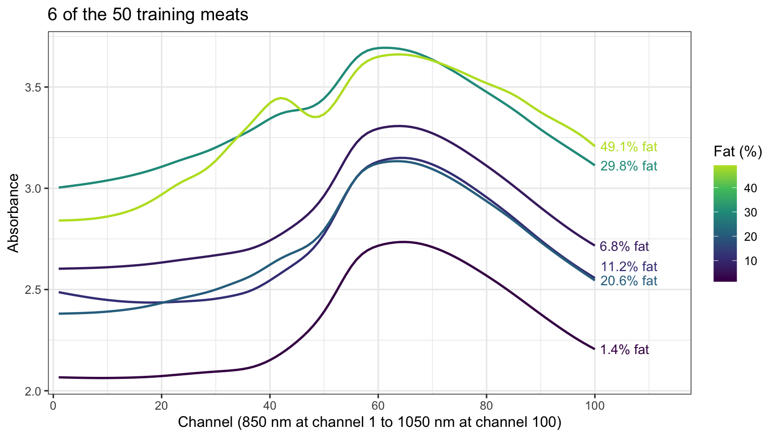
The training meats range from 1.4% to 49.1% fat. Every spectrum has the same shape, rising to a peak near channel 64 and falling after it, and the spectra differ mostly by a vertical shift. The shift is only loosely related to fat: over the training meats, the correlation of fat with a meat’s mean absorbance is 0.47. The fattest meats shown also have a bump or shoulder near channel 42 that the leaner ones lack. The fat content is in the details of the shape, which no single channel records.
25.1.2 Dimensions
Each channel’s absorbance is an explanatory variable, so there are \(p = 100\) candidate features for \(n = 50\) training meats. The channels are nearly copies of one another: over the training meats, every pair of channels has correlation at least 0.981, and adjacent channels at least 0.99985.
25.2 Least squares
25.2.1 Perfect fits
The least squares fit of fat on all 100 channels uses the \(n \times (p + 1)\) model matrix \(\mathbf{X}\), a column of ones and one column per channel. Its rank is at most \(n\), the number of rows. With \(p + 1 > n\) the \((p + 1) \times (p + 1)\) matrix \(\mathbf{X}^\top\mathbf{X}\) therefore has rank at most \(n < p + 1\), so it is singular. The normal equations are
\[\mathbf{X}^\top\mathbf{X}\,b = \mathbf{X}^\top y,\]
where
- \(b\) is a \((p + 1)\)-vector of candidate estimates, the intercept first, and
- \(y\) is the \(n\)-vector of the training responses, the fat contents.
With \(\mathbf{X}^\top\mathbf{X}\) singular they have no unique solution. If \(\hat\beta\) solves them, so does \(\hat\beta + v\) for every \(v\) with \(\mathbf{X}v = 0\), and these \(v\) form a space of dimension at least \(p + 1 - n\); every solution has the same fitted values \(\mathbf{X}\hat\beta\). When the rank is \(n\), the columns of \(\mathbf{X}\) span all of \(\mathbb{R}^n\), so \(y\) is itself a combination of them: the fitted values \(\hat y_i\) equal the responses, the training residual sum of squares \(RSS = \sum_{i=1}^n\left(y_i - \hat y_i\right)^2\) is 0, and the training \(R^2\) is 1.
# Least squares on all 100 channels.
all_formula <- reformulate(channels, response = "fat")
all_fit <- lm(all_formula, data = train)
all_estimates <- coef(all_fit)
n_na <- sum(is.na(all_estimates))
all_r2 <- summary(all_fit)$r.squared

# The last channel with an estimate.
last_estimated <- tail(names(all_estimates)[!is.na(all_estimates)], 1)
lm() returns estimates for the intercept and the first 49 channels, x_001 to x_049, and NA for the other 51. It has picked one of the infinitely many solutions by setting those 51 estimates to zero. The model matrix has rank 50, which is \(n\), and the training \(R^2\) is 1.0000.
25.2.2 Channel sweep
The perfect fit does not need all 100 channels: any \(n - 1 = 49\) channels with a model matrix of rank \(n\) give one. The sweep below fits least squares on the first \(d\) channels of a random ordering, for \(d = 1, \ldots, n - 1\), where \(d\) is the number of features in the model, as in the Subset Selection lecture. Adding channels in wavelength order would add, at each step, a channel with correlation at least 0.99985 with the one before it; a random order spreads the channels over the spectrum from the start.
NoteCode
# Mean squared error of predictions y_hat of responses y.
mse <- function(y, y_hat) {
  mean((y - y_hat)^2)
}

# A random ordering of the channels.
channel_order <- sample(p)

# Least squares on the first d channels of the ordering: training R^2,
# training and test MSE, the overall F-test, sigma-hat, and the number of
# estimates with p-value below 0.05.
sweep_fit <- function(d) {
  # Fit least squares to the first d channels.
  kept <- channels[channel_order[seq_len(d)]]
  fit <- lm(reformulate(kept, response = "fat"), data = train)
  fit_summary <- summary(fit)
  has_df <- fit$df.residual > 0

  # The overall F-test, when the fit has residual degrees of freedom.
  f_p <- NA_real_
  n_small <- NA_integer_
  if (has_df) {
    f <- fit_summary$fstatistic
    f_p <- pf(f[1], f[2], f[3], lower.tail = FALSE)
    slope_p <- fit_summary$coefficients[-1, "Pr(>|t|)"]
    n_small <- sum(slope_p < 0.05)
  }

  # Summaries of the fit, one row.
  slopes <- coef(fit)[-1]
  tibble(d = d,
         rank = fit$rank,
         slope_min = min(slopes),
         slope_max = max(slopes),
         r2 = fit_summary$r.squared,
         rss = sum(residuals(fit)^2),
         train_mse = mse(y_train, fitted(fit)),
         test_mse = mse(y_test, predict(fit, test)),
         f_p = unname(f_p),
         n_small = n_small,
         sigma_hat = if (has_df) sigma(fit) else NA_real_,
         aic = AIC(fit),
         bic = BIC(fit))
}
sweep_sizes <- seq_len(n_train - 1)
sweep_results <- map(sweep_sizes, sweep_fit) |>
  list_rbind()

# Every model matrix has full column rank d + 1.
stopifnot(all(sweep_results$rank == sweep_results$d + 1))

# The null model: the training mean predicts every test meat.
null_test_mse <- mse(y_test, mean(y_train))

# Axis of d: major lines every 10 channels from 0 to n, minor lines midway
# between them.
d_axis <- scale_x_continuous(breaks = seq(0, n_train, by = 10),
                             minor_breaks = seq(5, n_train - 5, by = 10))

# Log-scale axis of a mean squared error: major lines at powers of 10, minor
# lines midway between them in log space.
mse_powers <- 0:4
mse_axis <- scale_y_log10(breaks = 10^mse_powers,
                          minor_breaks = 10^(mse_powers + 0.5))

# Training R^2 against d.
sweep_title <- paste("Least squares on the first d channels,",
                     n_train, "training meats")
r2_plot <- ggplot(sweep_results, aes(x = d, y = r2)) +
  geom_line() +
  geom_point(size = 1.5) +
  d_axis +
  scale_y_continuous(breaks = seq(0.2, 1, by = 0.2),
                     minor_breaks = seq(0.3, 0.9, by = 0.2)) +
  labs(x = "Number of channels d",
       y = expression("Training " * R^2),
       title = sweep_title)

# Test MSE against d on a log scale, with the null model's.
null_label <- paste0("Null model: ", fmt(null_test_mse, 1))
test_plot <- ggplot(sweep_results, aes(x = d, y = test_mse)) +
  geom_hline(yintercept = null_test_mse, linetype = "dashed") +
  annotate("text",
           x = 1,
           y = null_test_mse,
           label = null_label,
           hjust = 0,
           vjust = -0.6) +
  geom_line() +
  geom_point(size = 1.5) +
  d_axis +
  mse_axis +
  labs(x = "Number of channels d",
       y = "Test MSE (log scale)",
       title = sweep_title)

# The d with the smallest test MSE, and the fit with d = n - 1.
d_best <- sweep_results$d[which.min(sweep_results$test_mse)]
last <- filter(sweep_results, d == n_train - 1)

# A d in the middle of the sweep, for prose.
d_mid <- 10

# The d with the smallest AIC() and BIC(), and those values as text.
d_aic <- sweep_results$d[which.min(sweep_results$aic)]
d_bic <- sweep_results$d[which.min(sweep_results$bic)]
as_text <- function(x) {
  if (is.infinite(x)) "$-\\infty$" else fmt(x, 1)
}
aic_text <- as_text(min(sweep_results$aic))
bic_text <- as_text(min(sweep_results$bic))
The tabs plot the training \(R^2\) and the test MSE of each fit against \(d\).
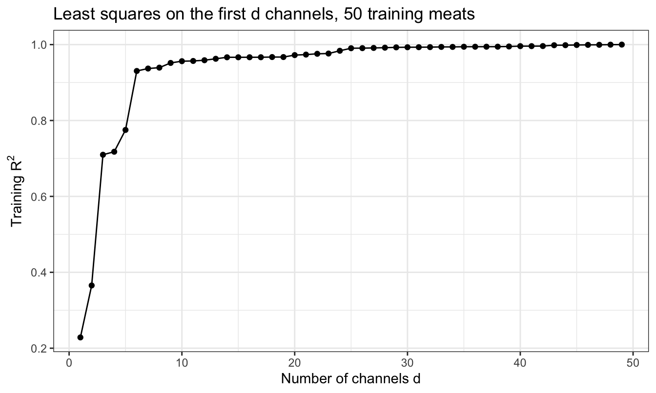
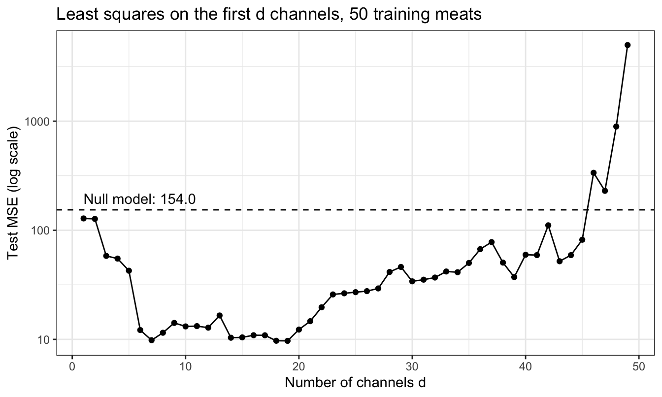
The training \(R^2\) rises with every channel added, from 0.228 with one channel to 0.956 with 10 and to 1 at \(d = 49\), where the training MSE is 0. The test MSE falls at first, to its smallest value, 9.69, at \(d = 19\), then climbs. At \(d = 49\) it is 4,988, 32 times the test MSE of the null model, 154.0, which predicts every meat by the training mean.
With \(d + 1 = n\) the fit passes through every training meat, so its fitted values carry all of the noise in the responses. Its estimates solve \(n\) equations in \(n\) unknowns whose columns are nearly copies of one another, and they run from −425,568 to 523,355 percentage points of fat per unit of absorbance. A test spectrum that differs slightly from the training spectra, in a direction in which the training spectra barely vary, is multiplied by these estimates. The training \(R^2\) cannot see any of this: it measures how well the fit reproduces the responses it was fit to.
25.2.3 Inference
NoteCode
# The largest d whose overall F-test has p-value below 0.01.
f_level <- 0.01
shown_fit <- sweep_results |>
  filter(f_p < f_level) |>
  slice_max(d)
d_shown <- shown_fit$d
The usual output of lm() does not warn of the failure either. At \(d = 46\), the largest \(d\) whose overall \(F\)-test of \(H_0: \beta_1 = \cdots = \beta_d = 0\) has \(p\)-value below 0.01, the \(p\)-value is 0.0016 and the training \(R^2\) is 0.9993, while none of the 46 individual estimates have a \(p\)-value below 0.05. The residual standard error is \(\hat\sigma = 1.49\) percentage points of fat, but the test MSE is 337, a root mean squared error of 18.3 percentage points and 2.2 times the test MSE of the null model.
Each of these numbers answers its own question. The \(F\)-test asks whether fat is related to the 46 channels at all, and it is. \(\hat\sigma\) estimates the standard deviation of the errors \(\epsilon_i\) in \(y_i = \beta_0 + \sum_{j=1}^d\beta_jx_{ij} + \epsilon_i\), not of the prediction errors, which add the variance of the estimates; with 3 residual degrees of freedom that variance is enormous. None of them estimates how well the fit predicts new meats.
25.2.4 Penalized criteria
\(C_p\) and BIC, from the subset selection lecture, are
\[C_p = \frac{1}{n}\left(RSS + 2d\hat\sigma^2\right), \qquad \text{BIC} = \frac{1}{n}\left[RSS + \log(n)\,d\hat\sigma^2\right],\]
with \(\sigma^2\) fixed at \(\hat\sigma^2\) from the model with all \(p\) candidate features: its RSS divided by its residual degrees of freedom, \(n - \text{rank}(\mathbf{X})\), which is \(n - p - 1\) only when \(\mathbf{X}\) has full column rank. With all \(p = 100\) channels, \(\text{rank}(\mathbf{X}) = n\), so the RSS and the residual degrees of freedom are both 0 and \(\hat\sigma^2 = 0/0\) is undefined. The largest model with a unique fit, \(d = n - 1\), is no help: its RSS is \(0\) with \(n - d - 1 = 0\) residual degrees of freedom. Setting \(\hat\sigma^2 = 0\) reduces \(C_p\) and BIC to \(RSS/n\), the training MSE, which is smallest, at 0, for the largest model. Any other estimate of \(\sigma^2\) would come from a smaller model, which would have to be chosen first.
The subset selection lecture’s AIC also fixes \(\sigma^2\) at \(\hat\sigma^2\), which makes it equivalent to \(C_p\), so it fails the same way. AIC() and BIC() in R use a different form: the Gaussian log-likelihood with \(\sigma^2\) estimated separately in each model by \(RSS/n\), so that \(-2\log L = n\log\left(2\pi RSS/n\right) + n\), plus a penalty of \(2\) or \(\log(n)\) per estimated parameter. As \(RSS \to 0\), \(-2\log L \to -\infty\) and no finite penalty offsets it. Over the sweep, AIC() is smallest at \(d = 49\), where it is \(-\infty\), and BIC() at \(d = 49\), where it is \(-\infty\). Once the training error can reach 0, none of the criteria can stop the search at a smaller model.
25.3 Regularization
25.3.1 Channels and fat
The figure plots, for the training meats, the correlation of fat with each channel’s absorbance.
NoteCode
# Correlation of fat with each channel over the training meats.
fat_cor <- drop(cor(X_train, y_train))
cor_data <- tibble(channel = seq_len(p), cor = fat_cor)
best_channel <- which.max(abs(fat_cor))

# Correlation against channel.
cor_plot <- ggplot(cor_data, aes(x = channel, y = cor)) +
  geom_line() +
  geom_point(size = 1.2) +
  channel_axis() +
  scale_y_continuous(limits = c(0.4, 0.55),
                     breaks = seq(0.4, 0.55, by = 0.05),
                     minor_breaks = seq(0.425, 0.525, by = 0.05)) +
  labs(x = "Channel",
       y = "Correlation with fat",
       title = paste(n_train, "training meats"))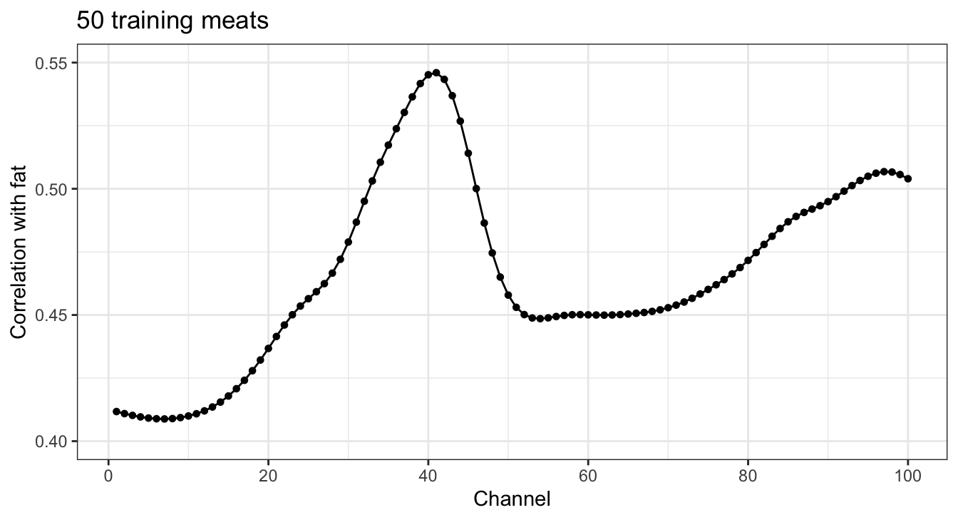
No channel predicts fat well alone: the correlations run from 0.409 to 0.546, at channel 41, so the best single channel explains 30% of the variance of fat in the training meats. The correlations change smoothly from channel to channel, as the channels themselves do. Predicting fat well needs a combination of many channels, and with \(p > n\) the combination must be constrained.
25.3.2 Four methods
The four methods of the earlier lectures constrain it, each fit to the 50 training meats with the standardized features \(\tilde x_{ij} = \left(x_{ij} - \bar x_j\right)/s_j\), where \(x_{ij}\) is the absorbance of meat \(i\) at channel \(j\) and \(\bar x_j\) and \(s_j\) are the mean and standard deviation (divisor \(n\)) of channel \(j\) over the training meats. \(\tilde{\mathbf{X}}\) is the \(n \times p\) matrix of standardized features, and \(\lambda \ge 0\) is a tuning parameter.
- Ridge regression minimizes \(RSS + \lambda\sum_{j=1}^p\beta_j^2\). For any \(\lambda > 0\) the matrix \(\tilde{\mathbf{X}}^\top\tilde{\mathbf{X}} + \lambda\mathbf{I}_p\), with \(\mathbf{I}_p\) the \(p \times p\) identity matrix, is positive definite, so the estimate is unique even with \(p > n\).
- The lasso minimizes \(RSS + \lambda\sum_{j=1}^p\left|\beta_j\right|\) and sets some estimates to exactly zero.
- Principal components regression (PCR) regresses fat on the first \(M\) principal component scores of the standardized features.
- Partial least squares (PLS) regresses fat on \(M\) directions chosen with the response.
Each of \(\lambda\) and \(M\) is chosen by 10-fold cross-validation on the folds drawn with the training sample, with the standardization, the principal components, and the PLS directions recomputed from the training folds in each fold.
25.3.3 Computation
glmnet() fits ridge regression and the lasso by coordinate descent, updating one estimate at a time, and stops when no update in a pass changes the criterion by more than a tolerance, its argument thresh, times the criterion of the null model. On these channels it meets that rule far from the minimum of the criterion, as the Test MSE subsection below shows; a tighter thresh and a larger maxit, the limit on passes, close the gap but can take minutes for each fit. So ridge regression uses its closed form,
\[\hat\beta^R_\lambda = \left(\tilde{\mathbf{X}}^\top\tilde{\mathbf{X}} + \lambda\mathbf{I}_p\right)^{-1}\tilde{\mathbf{X}}^\top\left(y - \bar y\mathbf{1}\right),\]
from the Ridge Regression lecture, where \(y\) is the \(n\)-vector of training responses, \(\bar y\) their mean, and \(\mathbf{1}\) the \(n\)-vector of ones, computed from the singular value decomposition of \(\tilde{\mathbf{X}}\). The lasso estimate is the \(\hat\beta^L_\lambda\) that satisfies, for every channel \(j\), the lasso conditions
\[\tilde{\mathbf{x}}_{\cdot j}^\top r = \frac{\lambda}{2}\,\text{sign}\left(\hat\beta^L_{\lambda j}\right) \quad \text{if } \hat\beta^L_{\lambda j} \ne 0, \qquad \left|\tilde{\mathbf{x}}_{\cdot j}^\top r\right| \le \frac{\lambda}{2} \quad \text{if } \hat\beta^L_{\lambda j} = 0,\]
where
- \(r = y - \bar y\mathbf{1} - \tilde{\mathbf{X}}\hat\beta^L_\lambda\) is the \(n\)-vector of residuals, and
- \(\tilde{\mathbf{x}}_{\cdot j}\) is column \(j\) of \(\tilde{\mathbf{X}}\), as in the PCR and PLS lecture.
The first condition sets the derivative of the criterion in \(\beta_j\) to zero; the second says that moving \(\beta_j\) away from zero in either direction would raise the penalty by more than it lowers the RSS. An active-set method solves the first condition exactly, as a linear system, on a set of nonzero estimates with fixed signs, and changes the set until the second holds for every other channel. Both fits work on this chapter’s \(\lambda\) directly, with no conversion to glmnet()’s.
NoteCode
# Standard deviation with divisor n.
sd_n <- function(v) {
  deviations <- v - mean(v)
  sqrt(mean(deviations^2))
}

# Standardize the columns of X with the given centers and scales.
standardize <- function(X, x_center, x_scale) {
  X_centered <- sweep(X, 2, x_center)
  sweep(X_centered, 2, x_scale, "/")
}

# Original-scale estimates, one column per lambda, from standardized-scale
# estimates B_std and the standardization of X and y.
original_scale <- function(B_std, X, y) {
  x_center <- colMeans(X)
  x_scale <- apply(X, 2, sd_n)
  b <- B_std / x_scale
  rbind(`(Intercept)` = mean(y) - colSums(b * x_center), b)
}

# Ridge estimates on the standardized scale for each lambda, from the
# singular value decomposition X_std = U D V'.
ridge_std <- function(X_std, y_centered, lambdas) {
  sv <- svd(X_std)
  shrink <- outer(sv$d, lambdas, function(d, l) d / (d^2 + l))
  u_y <- drop(crossprod(sv$u, y_centered))
  sv$v %*% (shrink * u_y)
}

# Lasso estimates on the standardized scale for each lambda, in decreasing
# order, by an active-set method. On the active set with signs s, the lasso
# conditions X_A'(y - X_A b_A) = (lambda / 2) s solve to a target; if the
# target keeps the signs it is the solution on that set, and a zero estimate
# whose condition |x_j'(y - X b)| <= lambda / 2 fails joins the set; if not,
# a line search to the target stops where the criterion is smallest and the
# estimates that reach zero there leave the set.
lasso_std <- function(X_std, y_centered, lambdas, max_steps = 1000) {
  p <- ncol(X_std)
  gram <- crossprod(X_std)
  xy <- drop(crossprod(X_std, y_centered))
  B <- matrix(0, p, length(lambdas))
  b <- numeric(p)

  # The criterion RSS + lambda * sum |b|.
  criterion <- function(b, lambda) {
    sum((y_centered - X_std %*% b)^2) + lambda * sum(abs(b))
  }

  for (k in seq_along(lambdas)) {
    half <- lambdas[k] / 2
    active <- which(b != 0)
    signs <- sign(b[active])
    converged <- FALSE

    for (step in seq_len(max_steps)) {
      if (length(active) > 0) {
        # Solve the conditions on the active set with these signs.
        gram_active <- gram[active, active, drop = FALSE]
        target <- drop(solve(gram_active, xy[active] - half * signs))

        # Signs change: line search to the target, then update the set.
        if (any(sign(target) != signs)) {
          direction <- numeric(p)
          direction[active] <- target - b[active]
          crossing <- -b[active] / direction[active]
          t_try <- c(crossing[crossing > 0 & crossing < 1], 1)
          values <- map_dbl(t_try, \(t) criterion(b + t * direction,
                                                  lambdas[k]))
          t_best <- t_try[which.min(values)]
          b <- b + t_best * direction
          b[active[crossing == t_best]] <- 0
          active <- which(b != 0)
          signs <- sign(b[active])
          next
        }
        b[] <- 0
        b[active] <- target
      }

      # The zero estimate whose condition fails by the most joins the set.
      gradient <- xy - drop(gram %*% b)
      excess <- abs(gradient) - half
      excess[active] <- -Inf
      if (max(excess) <= 1e-9 * half) {
        converged <- TRUE
        break
      }
      j <- which.max(excess)
      active <- c(active, j)
      signs <- c(signs, sign(gradient[j]))
    }

    stopifnot(converged)
    B[, k] <- b
  }
  B
}

# Ridge or lasso estimates on the original scale for each lambda.
penalized_path <- function(X, y, lambdas, std_fit) {
  x_center <- colMeans(X)
  x_scale <- apply(X, 2, sd_n)
  X_std <- standardize(X, x_center, x_scale)
  y_centered <- y - mean(y)
  B_std <- std_fit(X_std, y_centered, lambdas)
  original_scale(B_std, X, y)
}

# Grids of lambda, in decreasing order.
ridge_grid <- 10^seq(4, -8, length.out = 121)
lasso_grid <- 10^seq(3, -4, length.out = 71)

# Ridge and lasso paths for the data X and y.
ridge_path <- function(X, y) {
  penalized_path(X, y, ridge_grid, ridge_std)
}
lasso_path <- function(X, y) {
  penalized_path(X, y, lasso_grid, lasso_std)
}

# Both fit to the training meats.
B_ridge <- ridge_path(X_train, y_train)
B_lasso <- lasso_path(X_train, y_train)

# The standardized training features, for checking the lasso conditions.
x_center <- colMeans(X_train)
x_scale <- apply(X_train, 2, sd_n)
X_std <- standardize(X_train, x_center, x_scale)
y_centered <- y_train - mean(y_train)

# Largest failure of the lasso conditions over the grid, relative to
# lambda / 2.
condition_gap <- function(b_std, lambda) {
  gradient <- drop(crossprod(X_std, y_centered - X_std %*% b_std))
  nonzero <- b_std != 0
  on_set <- abs(gradient[nonzero] - lambda / 2 * sign(b_std[nonzero]))
  off_set <- pmax(abs(gradient[!nonzero]) - lambda / 2, 0)
  max(c(on_set, off_set, 0)) / (lambda / 2)
}
B_lasso_std <- B_lasso[-1, ] * x_scale
lasso_gaps <- map_dbl(seq_along(lasso_grid),
                      \(k) condition_gap(B_lasso_std[, k], lasso_grid[k]))
Over the 71 values of \(\lambda\) on the lasso grid, from \(10^{3}\) to \(10^{-4}\), the lasso conditions hold to within a fraction \(1.3 \times 10^{-5}\) of \(\lambda/2\).
25.3.4 Tuning
NoteCode
# Sums of squared errors of held-out fold l, for every value of the tuning
# parameter, from the estimates that path() computes from the training folds.
fold_sse <- function(l, path) {
  out <- fold_id == l
  B <- path(X_train[!out, ], y_train[!out])
  y_hat <- cbind(1, X_train[out, ]) %*% B
  colSums((y_train[out] - y_hat)^2)
}

# Cross-validation estimate for every value of the tuning parameter.
cv_estimate <- function(path) {
  sse <- sapply(seq_len(n_folds), fold_sse, path = path)
  rowSums(sse) / n_train
}

# Ridge regression and the lasso, and the lambda with the smallest estimate.
cv_ridge <- cv_estimate(ridge_path)
cv_lasso <- cv_estimate(lasso_path)
k_ridge <- which.min(cv_ridge)
k_lasso <- which.min(cv_lasso)
lambda_ridge <- ridge_grid[k_ridge]
lambda_lasso <- lasso_grid[k_lasso]

# PCR and PLS with up to M_max directions, cross-validated by pcr() and
# plsr() on the same folds; both standardize within each fold.
M_max <- 25
segments <- split(seq_len(n_train), fold_id)
pcr_fit <- pcr(all_formula,
               ncomp = M_max,
               data = train,
               scale = TRUE,
               validation = "CV",
               segments = segments)
pls_fit <- plsr(all_formula,
                ncomp = M_max,
                data = train,
                scale = TRUE,
                validation = "CV",
                segments = segments)
cv_of <- function(fit) {
  MSEP(fit, estimate = "CV", intercept = FALSE)$val[1, 1, ]
}
cv_pcr <- cv_of(pcr_fit)
cv_pls <- cv_of(pls_fit)
M_pcr <- which.min(cv_pcr)
M_pls <- which.min(cv_pls)

# Null model: the mean of the training folds predicts the held-out fold.
null_sse <- function(l) {
  out <- fold_id == l
  sum((y_train[out] - mean(y_train[!out]))^2)
}
cv_null <- sum(map_dbl(seq_len(n_folds), null_sse)) / n_train

# Shared look of the three tabs: the null model's estimate dashed, the
# chosen value circled, a log-scale estimate, and the same y limits, from the
# smallest estimate of any method to a little above the null model's.
cv_ylim <- c(min(cv_ridge, cv_lasso, cv_pcr, cv_pls), 1.1 * cv_null)
cv_axis_label <- paste0(n_folds, "-fold CV estimate (log scale)")
cv_title <- paste(n_train, "training meats")
cv_layers <- list(
  geom_hline(yintercept = cv_null, linetype = "dashed"),
  mse_axis,
  coord_cartesian(ylim = cv_ylim),
  labs(y = cv_axis_label, title = cv_title)
)

# Axis of lambda over both grids: major lines every 2 powers of 10, minor
# lines midway between them in log space.
lambda_axis <- scale_x_log10(breaks = 10^seq(-8, 4, by = 2),
                             minor_breaks = 10^seq(-9, 5, by = 2),
                             labels = scales::label_log())

# The estimate against lambda for one of ridge regression and the lasso.
lambda_cv_plot <- function(grid, cv, k_chosen) {
  chosen <- tibble(lambda = grid[k_chosen], cv = cv[k_chosen])
  ggplot(tibble(lambda = grid, cv = cv), aes(x = lambda, y = cv)) +
    cv_layers +
    geom_line() +
    geom_point(data = chosen, size = 4, shape = 1, color = "#D55E00") +
    lambda_axis +
    labs(x = expression(lambda ~ "(log scale)"),
         caption = "Circle: the chosen lambda. Dashed: the null model.")
}
ridge_cv_plot <- lambda_cv_plot(ridge_grid, cv_ridge, k_ridge)
lasso_cv_plot <- lambda_cv_plot(lasso_grid, cv_lasso, k_lasso)

# PCR and PLS against M, with the chosen M of each circled.
method_levels <- c("PCR", "PLS")
direction_cv <- tibble(method = factor(rep(method_levels, each = M_max),
                                       levels = method_levels),
                       M = rep(seq_len(M_max), 2),
                       cv = c(cv_pcr, cv_pls))
direction_chosen <- tibble(method = factor(method_levels,
                                           levels = method_levels),
                           M = c(M_pcr, M_pls),
                           cv = c(cv_pcr[M_pcr], cv_pls[M_pls]))
direction_cv_plot <- ggplot(direction_cv,
                            aes(x = M,
                                y = cv,
                                color = method,
                                linetype = method,
                                shape = method)) +
  cv_layers +
  geom_line() +
  geom_point(size = 2) +
  geom_point(data = direction_chosen,
             size = 5,
             shape = 1,
             show.legend = FALSE) +
  scale_color_manual(values = okabe_ito[c(5, 4)]) +
  scale_x_continuous(breaks = seq(0, M_max, by = 5),
                     minor_breaks = seq(2.5, M_max - 2.5, by = 5)) +
  labs(x = "Number of directions M",
       color = NULL,
       linetype = NULL,
       shape = NULL,
       caption = paste("Circles: the chosen M of each method.",
                       "Dashed: the null model.")) +
  theme(legend.position = "inside",
        legend.position.inside = c(0.99, 0.9),
        legend.justification = c(1, 1),
        legend.background = element_rect(color = "grey50"))

# Line up the panels of the three tabs: the lambda axes use expressions, whose
# labels are taller than the plain labels of the M axis.
cv_aligned <- patchwork::align_patches(ridge_cv_plot,
                                       lasso_cv_plot,
                                       direction_cv_plot)
ridge_cv_tab <- cv_aligned[[1]]
lasso_cv_tab <- cv_aligned[[2]]
direction_cv_tab <- cv_aligned[[3]]

# Principal component variances of the standardized training features, and
# ridge regression's factor v_m / (v_m + lambda / n) on each component.
v <- eigen(crossprod(X_std) / n_train,
           symmetric = TRUE,
           only.values = TRUE)$values
ridge_factor <- v / (v + lambda_ridge / n_train)
n_half <- sum(ridge_factor >= 0.5)

# Smallest estimate of each method.
cv_minima <- c(min(cv_ridge), min(cv_lasso), min(cv_pcr), min(cv_pls))

# Number of nonzero lasso estimates at the chosen lambda.
lasso_nonzero <- sum(B_lasso[-1, k_lasso] != 0)
The tabs plot \(\text{CV}_{(10)}\) against \(\lambda\) for ridge regression and the lasso and against \(M\) for PCR and PLS, each with the estimate for the null model as a dashed line.
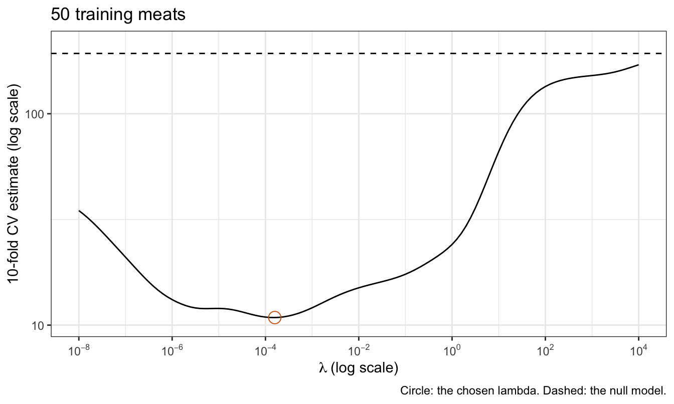
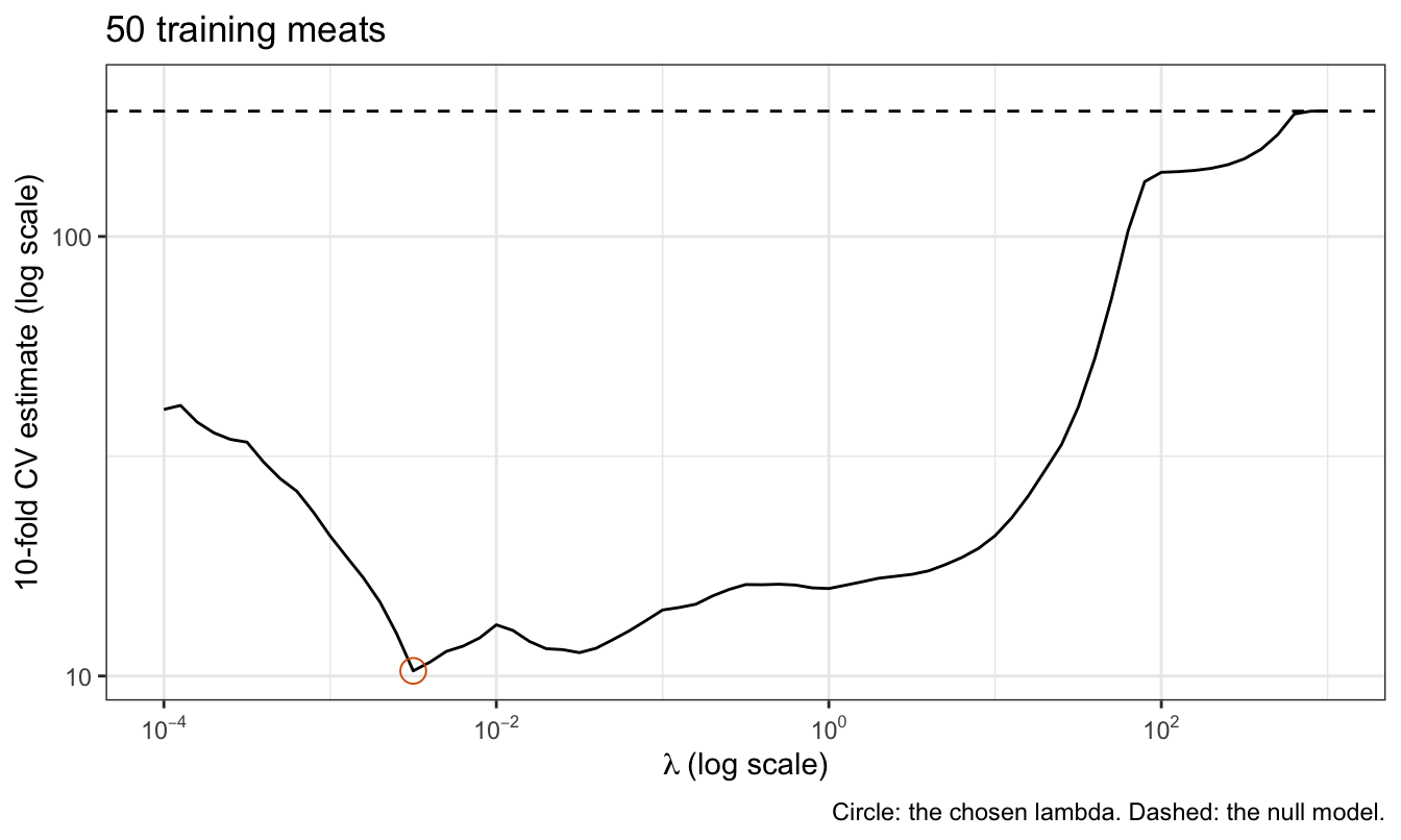
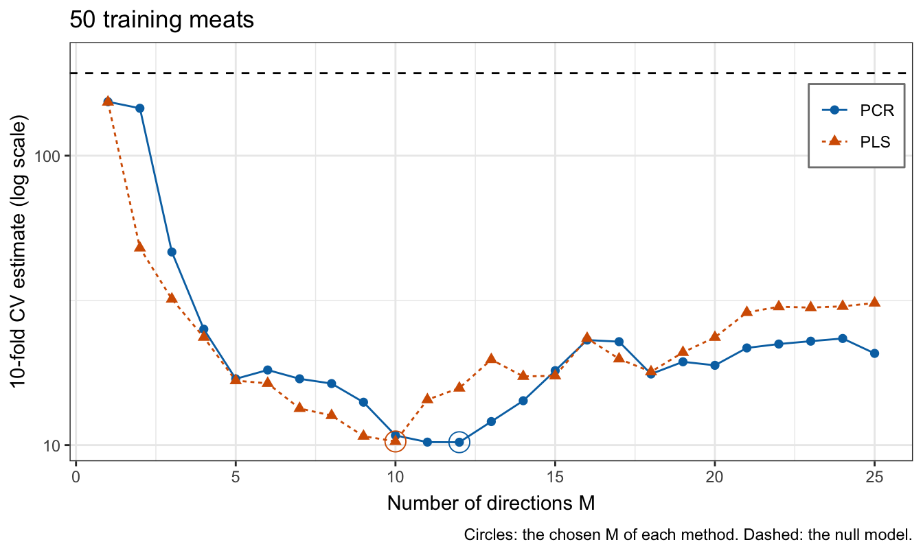
All four curves fall from the null model’s estimate, 192.8, to a minimum between 10.2 and 10.9 and rise again as the fit becomes more flexible.
- Ridge regression chooses \(\lambda = 1.6 \times 10^{-4}\). That is small in absolute terms, but the principal component variances \(v_m\) of the standardized channels fall from 99.3 for the first component to \(6.2 \times 10^{-7}\) for the 15th, and the factor \(v_m/(v_m + \lambda/n)\) of the PCR lecture keeps at least half of the term of the first 12 components and shrinks the rest toward zero.
- The lasso chooses \(\lambda = 3.2 \times 10^{-3}\), with 20 nonzero estimates. Its curve is jagged at small \(\lambda\), where channels enter and leave the active set.
- PCR chooses \(M = 12\) components and PLS \(M = 10\) directions.
25.3.5 Test MSE
Each method with its chosen tuning parameter, fit to all 50 training meats, and the null model are evaluated once on the 143 test meats.
NoteCode
# Test predictions of the four chosen fits.
ridge_pred <- drop(cbind(1, X_test) %*% B_ridge[, k_ridge])
lasso_pred <- drop(cbind(1, X_test) %*% B_lasso[, k_lasso])
pcr_pred <- predict(pcr_fit, test, ncomp = M_pcr)[, 1, 1]
pls_pred <- predict(pls_fit, test, ncomp = M_pls)[, 1, 1]

# Test MSE of each, and of the null model.
test_mse <- c(null = null_test_mse,
              ridge = mse(y_test, ridge_pred),
              lasso = mse(y_test, lasso_pred),
              pcr = mse(y_test, pcr_pred),
              pls = mse(y_test, pls_pred))

# Table of the tuning parameters, nonzero estimates, cross-validation
# estimates, and test MSE.
tuning_text <- c("",
                 paste0("$\\lambda = ", sci(lambda_ridge), "$"),
                 paste0("$\\lambda = ", sci(lambda_lasso), "$"),
                 paste0("$M = ", M_pcr, "$"),
                 paste0("$M = ", M_pls, "$"))
cv_values <- c(cv_null,
               cv_ridge[k_ridge],
               cv_lasso[k_lasso],
               cv_pcr[M_pcr],
               cv_pls[M_pls])
test_tibble <- tibble(Method = c("Null", "Ridge", "Lasso", "PCR", "PLS"),
                      tuning = tuning_text,
                      nonzero = c(0, p, lasso_nonzero, p, p),
                      cv = fmt(cv_values, 2),
                      test = fmt(test_mse, 2))
test_columns <- c("Method",
                  "Tuning",
                  "Nonzero",
                  paste0(n_folds, "-fold CV"),
                  "Test MSE")
test_table <- knitr::kable(test_tibble,
                           col.names = test_columns,
                           align = "llrrr")

# glmnet() at its defaults, at the chosen lambdas: lambda_glmnet is
# lambda * s_y / n for ridge regression and lambda / (2 n) for the lasso.
default_thresh <- formals(glmnet)$thresh
s_y <- sd_n(y_train)
glmnet_ridge <- glmnet(X_train,
                       y_train,
                       alpha = 0,
                       lambda = lambda_ridge * s_y / n_train)
glmnet_ridge_pred <- predict(glmnet_ridge, X_test)
glmnet_ridge_gap <- max(abs(glmnet_ridge_pred - ridge_pred))
glmnet_lasso <- glmnet(X_train,
                       y_train,
                       alpha = 1,
                       lambda = lasso_grid / (2 * n_train))
b_glmnet <- glmnet_lasso$beta[, k_lasso] * x_scale
lasso_criterion <- function(b_std, lambda) {
  sum((y_centered - X_std %*% b_std)^2) + lambda * sum(abs(b_std))
}
criterion_exact <- lasso_criterion(B_lasso_std[, k_lasso], lambda_lasso)
criterion_glmnet <- lasso_criterion(b_glmnet, lambda_lasso)
glmnet_lasso_pred <- predict(glmnet_lasso, X_test)[, k_lasso]
glmnet_lasso_test <- mse(y_test, glmnet_lasso_pred)

# glmnet() with a tight tolerance, which finishes in seconds for the lasso
# with lambda >= 1.
lasso_thresh <- 1e-12
lasso_maxit <- 1e9
large <- lasso_grid >= 1
glmnet_tight <- glmnet(X_train,
                       y_train,
                       alpha = 1,
                       lambda = lasso_grid[large] / (2 * n_train),
                       thresh = lasso_thresh,
                       maxit = lasso_maxit)
tight_pred <- predict(glmnet_tight, X_test)
exact_large <- cbind(1, X_test) %*% B_lasso[, large]
tight_gap <- max(abs(tight_pred - exact_large))

# Criteria of the tight glmnet() fit and the active-set fit at lambda = 1.
lambda_check <- 1
k_check <- which.min(abs(lasso_grid[large] - lambda_check))
b_tight <- glmnet_tight$beta[, k_check] * x_scale
b_exact <- B_lasso_std[, which(large)[k_check]]
criterion_tight <- lasso_criterion(b_tight, lambda_check)
criterion_check <- lasso_criterion(b_exact, lambda_check)

# The same check for ridge regression at lambda = 1.
ridge_thresh <- 1e-14
ridge_maxit <- 1e7
ridge_tight <- glmnet(X_train,
                      y_train,
                      alpha = 0,
                      lambda = lambda_check * s_y / n_train,
                      thresh = ridge_thresh,
                      maxit = ridge_maxit)
ridge_check <- penalized_path(X_train, y_train, lambda_check, ridge_std)
ridge_tight_pred <- predict(ridge_tight, X_test)
ridge_check_pred <- cbind(1, X_test) %*% ridge_check
ridge_tight_gap <- max(abs(ridge_tight_pred - ridge_check_pred))

# The methods with the smallest and largest test MSE, for prose.
method_names <- c(ridge = "ridge regression",
                  lasso = "the lasso",
                  pcr = "PCR",
                  pls = "PLS")
method_mse <- test_mse[names(method_names)]
best_method <- method_names[[names(which.min(method_mse))]]
worst_method <- method_names[[names(which.max(method_mse))]]
dense_mse <- method_mse[c("ridge", "pcr", "pls")]
dense_better <- all(dense_mse <= method_mse["lasso"])| Method | Tuning | Nonzero | 10-fold CV | Test MSE |
|---|---|---|---|---|
| Null | 0 | 192.81 | 153.95 | |
| Ridge | \(\lambda = 1.6 \times 10^{-4}\) | 100 | 10.86 | 8.09 |
| Lasso | \(\lambda = 3.2 \times 10^{-3}\) | 20 | 10.27 | 13.26 |
| PCR | \(M = 12\) | 100 | 10.23 | 8.71 |
| PLS | \(M = 10\) | 100 | 10.29 | 9.52 |
The table gives, for each method, its chosen tuning parameter, its number of nonzero estimates, its 10-fold cross-validation estimate, and its test MSE. On this training sample every method predicts the test meats far better than the null model: their test MSEs are 8.1 to 13.3, against 154.0, and against 4,988 for least squares on 49 channels. The ordering among them, with ridge regression best and the lasso worst, holds on this training sample of 50 meats; another training sample could rank them differently, and one training sample cannot show which method is best on average.
The default glmnet() fits would have told a different story about which channels the lasso uses. At the chosen \(\lambda\), the default lasso fit, with thresh = 1e-7, has 99 nonzero estimates, against 20 for the active-set fit, and a criterion 2.5 times the minimum, although its test MSE, 9.93, is lower than the active-set fit’s, 13.26: a fit that stops far from the lasso’s minimum keeps almost every channel, and on this training sample dense fits predict better. With neighboring channels correlated at least 0.99985, a change to one estimate in a pass of coordinate descent is almost undone by the change to its neighbor, so each update lowers the criterion little and the stopping rule is met early. The default ridge fit’s predictions of the test meats differ from the closed form by up to 5.8 percentage points.
A much tighter tolerance brings glmnet() close to the exact fits. With thresh = 1e-12 and maxit = 1e9, its lasso fits for \(\lambda \ge 1\) predict the test meats to within 0.050 of the active-set fits; the remaining gap is glmnet()’s, since at \(\lambda = 1\) its criterion is 714.9403 against 714.9391 for the active-set fit. With thresh = 1e-14 and maxit = 1e7, its ridge fit at \(\lambda = 1\) predicts the test meats to within \(3.1 \times 10^{-4}\) of the closed form.
25.3.6 Selected channels
The lasso chose 20 channels. The figure marks the channels with a nonzero estimate in the lasso fit, at the chosen \(\lambda\), to all 50 training meats and to the training folds of each fold, 45 meats each.
NoteCode
# Channels with a nonzero lasso estimate at the chosen lambda, fit to the
# training meats outside fold l.
fold_selected <- function(l) {
  out <- fold_id == l
  B <- lasso_path(X_train[!out, ], y_train[!out])
  which(B[-1, k_lasso] != 0)
}
selected_folds <- map(seq_len(n_folds), fold_selected)
selected_all <- which(B_lasso[-1, k_lasso] != 0)

# One row per fit and selected channel.
fit_labels <- c(paste("All", n_train, "training meats"),
                paste("Without fold", seq_len(n_folds)))
selected_data <- tibble(fit = fit_labels,
                        channel = c(list(selected_all), selected_folds)) |>
  unnest(channel) |>
  mutate(fit = factor(fit, levels = rev(fit_labels)),
         in_all = channel %in% selected_all)

# A tile for each selected channel, shaded by whether the fit to all the
# training meats selects it too.
in_all_labels <- c(`TRUE` = "Also selected with all training meats",
                   `FALSE` = "Not selected with all training meats")
selected_plot <- ggplot(selected_data,
                        aes(x = channel, y = fit, fill = in_all)) +
  geom_tile(width = 0.9, height = 0.8) +
  scale_fill_manual(values = c(`TRUE` = "grey20", `FALSE` = "#E69F00"),
                    labels = in_all_labels) +
  channel_axis(limits = c(0.5, p + 0.5)) +
  labs(x = "Channel",
       y = NULL,
       fill = NULL,
       title = "Lasso at the chosen lambda") +
  theme(legend.position = "bottom",
        panel.grid.minor = element_blank())

# Channels selected in every fit, and in any fit.
selected_every <- Reduce(intersect, selected_folds) |>
  intersect(selected_all)
selected_any <- Reduce(union, selected_folds) |>
  union(selected_all)
n_distinct_sets <- length(unique(map(c(list(selected_all), selected_folds),
                                     sort)))

# Test MSE of each fold's lasso fit.
fold_test_mse <- function(l) {
  out <- fold_id == l
  B <- lasso_path(X_train[!out, ], y_train[!out])
  mse(y_test, cbind(1, X_test) %*% B[, k_lasso])
}
fold_tests <- map_dbl(seq_len(n_folds), fold_test_mse)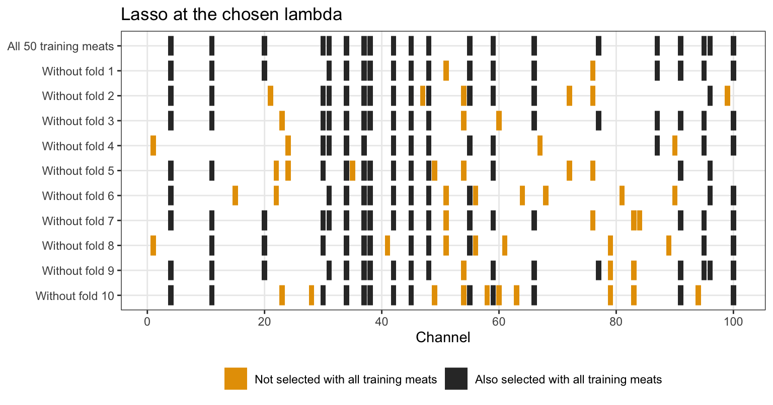
The 11 fits select 11 different sets of channels, of 16 to 23 channels each. Only 3 channels are selected by every fit, and 51 of the 100 channels are selected by at least one. Every pair of channels has correlation at least 0.981, so the lasso’s choice among them turns on small differences among the training meats in each fold.
The selected set is therefore one of many sets that predict fat, not the set of wavelengths at which fat absorbs. The fold fits, with their different sets, have test MSEs from 10.7 to 30.6; ridge regression, PCR, and PLS give every channel a nonzero estimate and, on this training sample, predict the test meats better than the lasso. The Lasso lecture found the same instability across repeated training samples; here it appears across the folds of a single training sample. A channel the lasso drops is not shown to be unrelated to fat.
NoteBeyond this course
- Minimum-norm interpolation. As \(\lambda \to 0\) with \(p > n\), the ridge estimate approaches the least squares solution with the smallest \(\sum_j\beta_j^2\), one of the infinitely many perfect fits. Unlike the perfect fits of the sweep, it can predict well, and the test MSE of such fits can fall again as \(p\) grows past \(n\), a pattern called double descent.
- Inference after selection. Methods for valid \(p\)-values and confidence intervals for the features a lasso selects, such as selective inference and sample splitting, condition on or avoid the selection.
- Grouped and smooth penalties. The elastic net, which adds a ridge penalty to the lasso, tends to select correlated features together, and penalties on differences between neighboring estimates suit features ordered along a spectrum.
- Lasso algorithms. Least angle regression computes the whole lasso path exactly by following it from one change of the active set to the next.
25.4 Conclusion
When the number of features \(p\) is close to or above the number of training observations \(n\), least squares fails. With \(p + 1 > n\) the matrix \(\mathbf{X}^\top\mathbf{X}\) is singular, the normal equations have infinitely many solutions, and when \(\mathbf{X}\) has rank \(n\) every one of them fits the training responses exactly, with training RSS 0 and training \(R^2 = 1\). As the number of features approaches \(n\), the training error falls toward zero while the test error rises sharply, because the fit reproduces the noise and its estimates on correlated features become huge.
The quantities that describe a least squares fit cannot choose among such fits. The training \(R^2\) and the training MSE always improve with more features. The overall \(F\)-test and \(\hat\sigma\) answer other questions, and a small \(p\)-value can accompany a fit that predicts worse than the null model. \(C_p\), BIC, and AIC with \(\sigma^2\) fixed at the estimate from the model with all \(p\) features need that estimate, which is \(0/0\) when \(p \ge n - 1\); setting it to 0 turns them into the training MSE. AIC and BIC with \(\sigma^2\) estimated in each model go to \(-\infty\) at a perfect fit.
Ridge regression, the lasso, PCR, and PLS constrain the fit, and a tuning parameter chosen by \(k\)-fold cross-validation on the training data decides how much. Every data-dependent step of the fit, such as the standardization and the PCR and PLS directions, is recomputed from the training folds inside each fold; the chosen model is then refit to all the training data and evaluated once on test data. When the features are highly correlated, many different sets of features can predict about equally well, so the set the lasso selects changes from fold to fold within a training sample and does not identify the features that matter.
The next lecture compares subset selection, ridge regression, the lasso, PCR, and PLS across repeated training samples, to see which of them predicts best on average and how much the answer depends on the data.