# All home sales, their explanatory variables, and which are categorical.
ames <- modeldata::ames
n_all <- nrow(ames)
explanatory <- setdiff(names(ames), "Sale_Price")
is_categorical <- map_lgl(ames[explanatory], is.factor)
n_numeric <- sum(!is_categorical)
n_categorical <- sum(is_categorical)
n_levels <- map_int(ames[explanatory][is_categorical], nlevels)

# Columns of the model matrix with one dummy variable for every level but
# the first of every categorical variable, without the intercept.
all_matrix <- model.matrix(Sale_Price ~ ., data = ames)
n_all_columns <- ncol(all_matrix) - 1

# The rule of the data's compiler: remove every home with more than
# max_area square feet of above-ground living area.
max_area <- 4000
big_homes <- filter(ames, Gr_Liv_Area > max_area)
n_big <- nrow(big_homes)
big_partial <- filter(big_homes, Sale_Condition == "Partial")
big_other <- filter(big_homes, Sale_Condition != "Partial")

# BsmtFin_SF_1 against BsmtFin_Type_1: each value of the first goes with
# exactly one level of the second.
code_table <- table(ames$BsmtFin_SF_1, ames$BsmtFin_Type_1)
stopifnot(all(rowSums(code_table > 0) == 1))

# Missing values: none is NA, but a frontage of 0 marks a missing one.
stopifnot(!anyNA(ames))
n_no_frontage <- sum(ames$Lot_Frontage == 0)

# The homes analyzed: large homes removed, BsmtFin_SF_1 dropped, an
# indicator of a missing frontage added, and the log price.
homes <- ames |>
  filter(Gr_Liv_Area <= max_area) |>
  select(-BsmtFin_SF_1) |>
  mutate(Frontage_Missing = as.integer(Lot_Frontage == 0),
         log_price = log(Sale_Price))
n_homes <- nrow(homes)

# Sale price against living area, the removed homes on top.
status_levels <- c("Kept", "Removed")
cleaning_data <- ames |>
  mutate(status = if_else(Gr_Liv_Area > max_area, "Removed", "Kept"),
         status = factor(status, levels = status_levels)) |>
  arrange(status)

# Price on a log scale: major lines at every doubling from $12,500, minor
# lines midway between them in log space.
price_breaks <- 12500 * 2^(0:6)
price_axis <- scale_y_log10(breaks = price_breaks,
                            minor_breaks = price_breaks * sqrt(2),
                            labels = scales::label_dollar())

# Living area: major lines every 1,000 square feet, minor lines midway.
area_axis <- scale_x_continuous(breaks = seq(0, 6000, by = 1000),
                                minor_breaks = seq(500, 6500, by = 1000))
cleaning_plot <- ggplot(cleaning_data, aes(x = Gr_Liv_Area, y = Sale_Price,
                                           color = status, shape = status)) +
  geom_vline(xintercept = max_area, linetype = "dashed", color = "grey50") +
  geom_point(alpha = 0.5, size = 1) +
  scale_color_manual(values = c("grey40", okabe_ito[4])) +
  scale_shape_manual(values = c(16, 17)) +
  area_axis +
  price_axis +
  labs(x = "Above-ground living area (sq ft)", y = "Sale price (log scale)",
       color = NULL, shape = NULL, title = paste(big(n_all), "homes")) +
theme(legend.position = "bottom")26 Method Comparison
TipLearning objectives
After this lecture you should be able to
- compare least squares, forward stepwise selection, ridge regression, the lasso, PCR, and PLS by what each does to the features and the estimates (keeps some features and drops the rest, shrinks every estimate, shrinks and sets some to zero, or regresses on a few directions), by whether it selects features, and by its tuning parameter,
- carry out the choice of each method’s tuning parameter, \(d\), \(\lambda\), or \(M\), by \(k\)-fold cross-validation on the training sample, with the standardization, the forward stepwise path, and the PCR and PLS directions recomputed from the training folds in each fold, and evaluate the chosen fits once on test data,
- explain why the test MSEs of one training sample cannot rank the methods, and interpret a comparison over repeated training samples: the distribution of each method’s test MSE, the share of samples each method wins, and its median change relative to least squares,
- explain what the lasso and forward stepwise selection do with the dummy variables of a categorical explanatory variable,
- explain why the cross-validation estimate of a chosen fit can differ from its test MSE in either direction: choosing the smallest estimate makes it optimistic, while fitting each fold to fewer training observations raises it, most for least squares, and
- state, from the reasoning of the earlier lectures, the setting in which each method is expected to predict best, and explain why one dataset cannot establish those expectations.
The earlier lectures of this chapter gave five ways to control the flexibility of least squares, which fits every feature without restraint. Subset selection keeps some features and drops the rest. Ridge regression and the lasso keep the model and shrink its estimates. Principal components regression (PCR) and partial least squares (PLS) regress on a few linear combinations of the features. Each lecture used its own data. This lecture fits all six to one training sample and compares them.
26.1 Ames home sales
26.1.1 Data
Question. From a small training sample of home sales, which of the six methods predicts the sale price of a home best, and what does each give up?
Data. modeldata::ames, the data of the Cross-Validation in Practice lecture, records 2,930 home sales in Ames, Iowa, from 2006 to 2010. Each observation is a home. The response is the sale price, Sale_Price, in dollars. That lecture used six explanatory variables; this one uses all of them.
NoteCode
There are 33 numeric explanatory variables (areas, counts of rooms and baths, years, and the home’s Longitude and Latitude) and 40 categorical ones, with 2 to 29 levels; Neighborhood has 29. With one dummy variable for every level but one, they give 276 columns. The figure plots the sale price of every home against its above-ground living area.
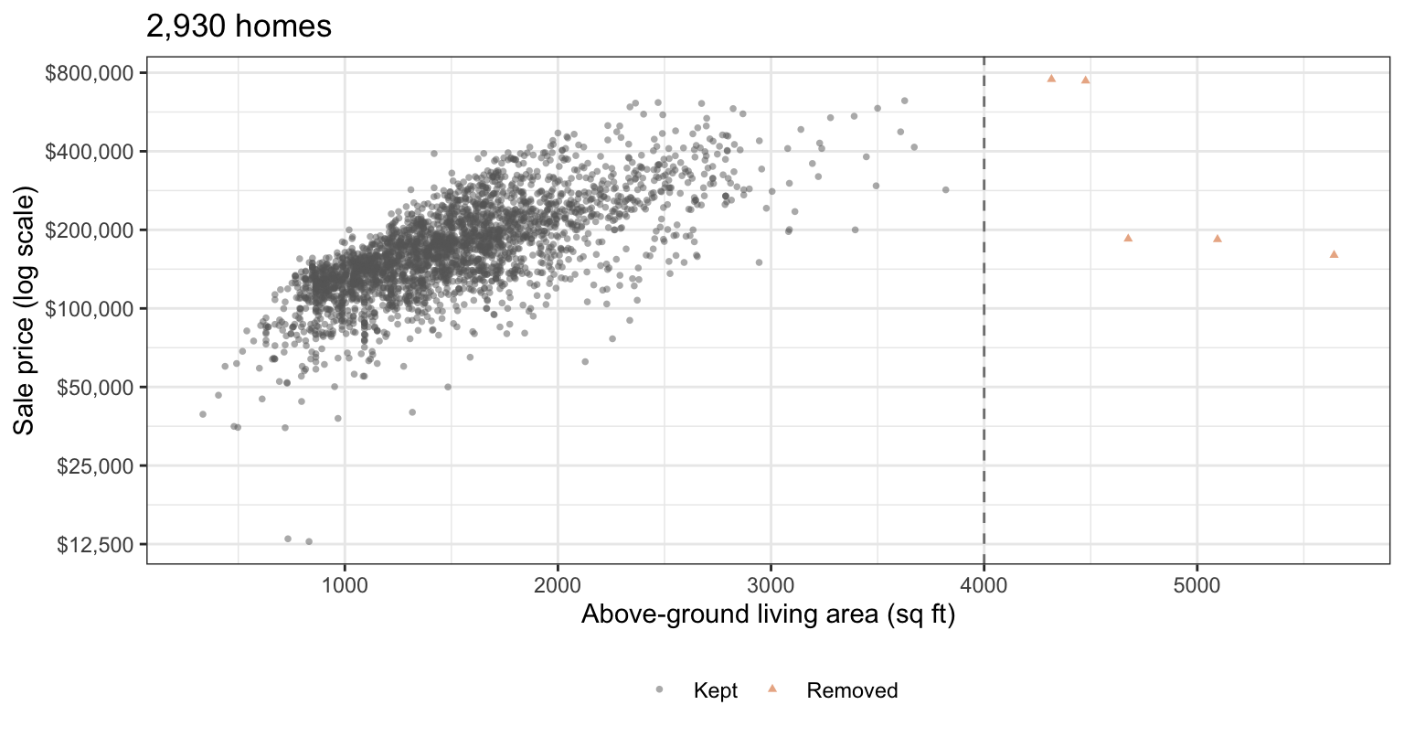
On the log scale price rises roughly linearly with living area. 5 homes have more than 4,000 square feet. 3 of them are partial sales, recorded before the home was complete, and sold for $160,000, $183,850, and $184,750, far below the trend; the other 2 sold for $745,000 and $755,000. The data’s compiler, De Cock (2011), “Ames, Iowa: Alternative to the Boston Housing Data as an End of Semester Regression Project,” Journal of Statistics Education 19(3), recommends removing every home with more than 4,000 square feet before modeling these data. That rule, applied here, leaves 2,925 homes, and every prediction below is for a home of at most 4,000 square feet.
Three more decisions shape the explanatory variables.
- A coded variable.
BsmtFin_SF_1is not an area: each of its values goes with exactly one level ofBsmtFin_Type_1, so it recodes that categorical variable as a number. It is dropped. - Missing values. No value is
NA, butLot_Frontage, the length of street along the lot, is 0 for 490 homes, whose frontage is missing in the original records. An indicator feature,Frontage_Missing, is added, so those homes are not treated as having no frontage. Levels such asNo_BasementandNo_Garagerecord an absence, not a missing value. - Ratings.
Overall_Cond,Heating_QC,Exter_Cond, and other ratings have levels in an order, butmodeldatastores them as unordered factors. They enter, like every categorical explanatory variable, as one dummy variable per level, which assumes nothing about the spacing of the levels.
Every model is linear in these features, with no interactions.
26.1.2 Training homes
# The training sample size.
n_train <- 200

# Training homes: a random sample; every other home is a test home.
train_id <- sample(n_homes, n_train)
train <- homes[train_id, ]
test <- homes[-train_id, ]
n_test <- nrow(test)

# Folds for 10-fold cross-validation of the training homes.
n_folds <- 10
fold_labels <- rep(seq_len(n_folds), length.out = n_train)
fold_id <- sample(fold_labels)
These sample() calls are the first random draws after set.seed(20261028). That leaves a training sample of 200 homes and 2,725 test homes, set aside until the chosen fits are evaluated. The training sample is small on purpose, for the reason given in the Candidate features subsection. The tabs plot the distribution of the sale price of the training homes, on the dollar and log scales, and the log price against three explanatory variables.
NoteCode
# Sale price and log sale price of the training homes, one panel each.
title_train <- paste(n_train, "training homes")
scale_labels <- c(Sale_Price = "Sale price (dollars)",
                  log_price = "Log sale price, log(dollars)")
response_long <- train |>
  select(Sale_Price, log_price) |>
  pivot_longer(everything(), names_to = "scale") |>
  mutate(scale = factor(scale_labels[scale], levels = scale_labels))

# Axis labels: dollars on the price panel, plain numbers on the log panel.
price_or_log <- function(x) {
  if (max(x, na.rm = TRUE) > 100) {
    scales::dollar(x)
  } else {
    as.character(x)
  }
}

# Grid lines every `step` across a panel's limits, starting at a multiple of
# the step; shift = step / 2 gives the minor lines midway between them.
lines_every <- function(limits, step, shift = 0) {
  from <- floor(limits[1] / step) * step + shift
  seq(from, limits[2] + step, by = step)
}

# Major lines every $200,000 on the price panel and every 0.5 on the log
# panel, minor lines midway.
response_step <- function(limits) {
  if (limits[2] > 100) 2e5 else 0.5
}
response_breaks <- function(limits) {
  lines_every(limits, response_step(limits))
}
response_minor <- function(limits) {
  step <- response_step(limits)
  lines_every(limits, step, shift = step / 2)
}

# Number of homes: major lines every 10 homes, minor lines midway.
response_plot <- ggplot(response_long, aes(x = value)) +
  geom_histogram(bins = 25, fill = "grey70", color = "grey30") +
  facet_wrap(~ scale, scales = "free_x") +
  scale_x_continuous(breaks = response_breaks,
                     minor_breaks = response_minor,
                     labels = price_or_log) +
  scale_y_continuous(breaks = seq(0, 50, by = 10),
                     minor_breaks = seq(5, 55, by = 10)) +
  labs(x = NULL, y = "Number of homes", title = title_train)

# Mean and median price of the training homes.
price_mean <- mean(train$Sale_Price)
price_median <- median(train$Sale_Price)

# Log price against three explanatory variables, one panel each.
three_labels <- c(Gr_Liv_Area = "Living area (sq ft)",
                  Year_Built = "Year built",
                  Total_Bsmt_SF = "Basement area (sq ft)")
three_long <- train |>
  select(log_price, all_of(names(three_labels))) |>
  pivot_longer(-log_price, names_to = "variable") |>
  mutate(variable = factor(three_labels[variable], levels = three_labels))

# Major lines every 20 years on the year panel, the only one whose limits
# exceed 1,000, and every 500 square feet on the area panels; minor lines
# midway.
three_step <- function(limits) {
  if (limits[1] > 1000) 20 else 500
}
three_breaks <- function(limits) {
  lines_every(limits, three_step(limits))
}
three_minor <- function(limits) {
  step <- three_step(limits)
  lines_every(limits, step, shift = step / 2)
}

# Log sale price: major lines every 0.5, minor lines midway.
log_price_axis <- scale_y_continuous(breaks = seq(10, 14, by = 0.5),
                                     minor_breaks = seq(10.25, 14, by = 0.5))
three_plot <- ggplot(three_long, aes(x = value, y = log_price)) +
  geom_point(alpha = 0.6, size = 1) +
  facet_wrap(~ variable, scales = "free_x") +
  scale_x_continuous(breaks = three_breaks,
                     minor_breaks = three_minor) +
  log_price_axis +
  labs(x = NULL, y = "Log sale price", title = title_train)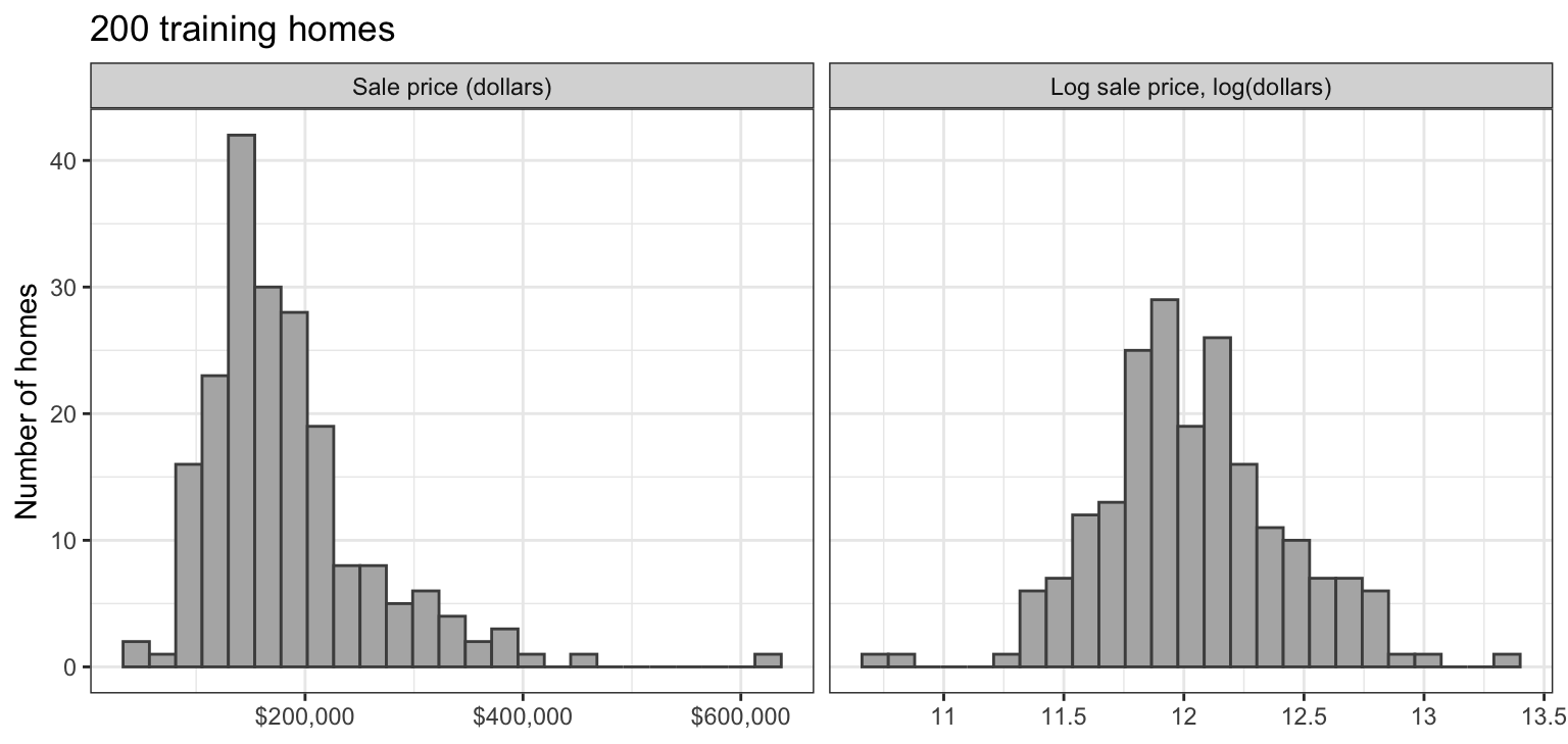
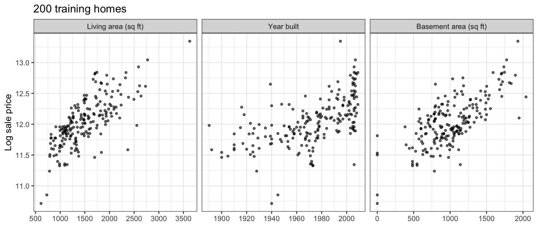
Sale price is right skewed: the mean training price, $182,460, is above the median, $165,000. Log price is close to symmetric, and it rises roughly linearly with living area, year built, and basement area; the stripe at zero basement area is the homes without a basement. Because the spread of log price is closer to constant, and an error on the log scale is a relative error in price, the response is the natural logarithm of the sale price,
\[y_i = \log\left(\texttt{Sale\_Price}_i\right),\]
where
- \(y_i\) is the response of home \(i\), and
- \(\texttt{Sale\_Price}_i\) is its sale price in dollars.
The Cross-Validation in Practice lecture used \(\log_{10}\), which multiplies every log by the same constant and changes no comparison. Every MSE below is in squared log dollars.
26.1.3 Candidate features
The figure counts, for every level of every categorical variable, the training homes that have it.
NoteCode
# Smallest number of training homes a level needs to keep its own dummy.
min_homes <- 5

# Number of training homes with each level of each categorical variable.
categorical <- explanatory[is_categorical]
level_counts <- map(categorical, \(v) {
  counts <- table(train[[v]])
  tibble(variable = v, level = names(counts), homes = as.vector(counts))
}) |>
  list_rbind()
n_level_total <- nrow(level_counts)
n_level_zero <- sum(level_counts$homes == 0)
n_level_rare <- sum(level_counts$homes > 0 & level_counts$homes < min_homes)

# Histogram of the counts of the levels that occur, on a log scale.
level_title <- paste(n_level_total - n_level_zero,
                     "levels that occur among the", title_train)
level_caption <- paste("Dashed line: levels to its left have fewer than",
                       min_homes, "training homes.")

# Homes on a log scale: major lines at powers of 2, minor lines midway
# between them in log space, at the edges of the histogram's bins.
homes_powers <- 0:7
homes_axis <- scale_x_log10(breaks = 2^homes_powers,
                            minor_breaks = 2^(homes_powers - 0.5))

# Number of levels: major lines every 5 levels, minor lines midway.
levels_axis <- scale_y_continuous(breaks = seq(0, 30, by = 5),
                                  minor_breaks = seq(2.5, 32.5, by = 5))
level_plot <- level_counts |>
  filter(homes > 0) |>
  ggplot(aes(x = homes)) +
  geom_histogram(breaks = 2^(-0.5 + 0:16 / 2), fill = "grey70",
                 color = "grey30") +
  geom_vline(xintercept = min_homes - 0.5, linetype = "dashed",
             color = okabe_ito[4]) +
  homes_axis +
  levels_axis +
  labs(x = "Training homes with the level (log scale)",
       y = "Number of levels", title = level_title, caption = level_caption)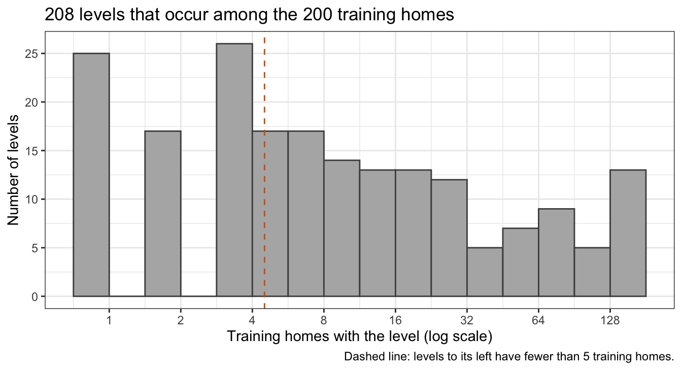
With 200 training homes, many levels are rare: of the 283 levels, 75 occur in no training home and 68 in one to 4. A dummy variable for a level with one or two training homes would have an estimate set by those homes alone. The features are therefore built from the training homes by three rules.
- Rare levels. The most common level of each categorical variable among the training homes is its reference, and a level with fewer than 5 training homes joins the reference. As in the Subset Selection lecture, merging a level into the reference is what dropping its dummy variable does; here a rule that uses no sale prices does it before any fit. A categorical variable left with only its reference contributes no feature.
- Dummy variables. Each remaining level other than the reference gets a dummy variable, and the numeric explanatory variables, with
Frontage_Missing, enter as recorded. - Redundant columns. A column that is constant among the training homes, or an exact linear combination of the intercept and the columns before it, is dropped, as
Doorswas in the Subset Selection lecture.
NoteCode
# Levels kept for a categorical variable: the most common level among the
# sample's homes first, as the reference, then every other level with at
# least min_homes of those homes.
kept_levels <- function(x, min_homes) {
  counts <- table(x)
  by_size <- names(counts)[order(-counts)]
  common <- by_size[counts[by_size] >= min_homes]
  union(by_size[1], common)
}

# x with every level outside `levels` merged into the reference, levels[1].
recode_levels <- function(x, levels) {
  x <- as.character(x)
  x[!(x %in% levels)] <- levels[1]
  factor(x, levels = levels)
}

# Feature matrices of the sample's homes and of new homes, built by the
# three rules from the sample's explanatory variables alone.
make_features <- function(sample_homes, new_homes, min_homes = 5) {
  # Explanatory variables only.
  x_sample <- select(sample_homes, -Sale_Price, -log_price)
  x_new <- select(new_homes, -Sale_Price, -log_price)

  # Rule 1: merge rare levels into the reference.
  factors <- names(x_sample)[map_lgl(x_sample, is.factor)]
  levels_kept <- map(x_sample[factors], kept_levels, min_homes = min_homes)
  for (v in factors) {
    x_sample[[v]] <- recode_levels(x_sample[[v]], levels_kept[[v]])
    x_new[[v]] <- recode_levels(x_new[[v]], levels_kept[[v]])
  }
  one_level <- factors[lengths(levels_kept) == 1]
  x_sample <- select(x_sample, -all_of(one_level))
  x_new <- select(x_new, -all_of(one_level))

  # Rule 2: dummy variables; column 1 is the intercept.
  X_sample <- model.matrix(~ ., data = x_sample)
  X_new <- model.matrix(~ ., data = x_new)

  # Rule 3: keep the columns that QR with pivoting finds independent of the
  # intercept and the columns before them.
  qr_sample <- qr(X_sample, tol = 1e-7)
  independent <- sort(qr_sample$pivot[seq_len(qr_sample$rank)])
  stopifnot(independent[1] == 1)
  keep <- independent[-1]
  list(X = X_sample[, keep, drop = FALSE],
       X_new = X_new[, keep, drop = FALSE],
       X_all = X_sample[, -1, drop = FALSE],
       one_level = one_level,
       dropped = colnames(X_sample)[-independent])
}

# The features of the training and the test homes.
features <- make_features(train, test, min_homes)
X_train <- features$X
X_test <- features$X_new
y_train <- train$log_price
y_test <- test$log_price
p <- ncol(X_train)

# Dropped columns that are constant, and those that repeat a kept column.
dropped_columns <- features$X_all[, features$dropped, drop = FALSE]
is_constant <- apply(dropped_columns, 2, \(x) all(x == x[1]))
repeats_kept <- apply(dropped_columns, 2, \(x) {
  any(colSums(abs(X_train - x)) == 0)
})

# The prose names one constant column and says every other one repeats a
# kept column.
stopifnot(sum(is_constant) == 1,
          all(repeats_kept[!is_constant]))
Rule 1 leaves 34 of the 40 categorical variables with a dummy variable; rule 2 gives 133 columns, and rule 3 drops 11 of them: Bldg_TypeTwoFmCon, Bldg_TypeDuplex, House_StyleSLvl, Exterior_2ndCmentBd, Bsmt_ExposureNo_Basement, BsmtFin_Type_1No_Basement, BsmtFin_Type_2No_Basement, Garage_FinishNo_Garage, Garage_CondNo_Garage, Pool_Area, and Sale_ConditionPartial. Pool_Area is constant among the training homes, and the other 10 each repeat a kept column exactly: several categorical variables record the same fact, such as the absence of a basement or the type of building. That leaves \(p = 122\) candidate features for \(n = 200\) training homes, where
- \(n\) is the number of training homes, indexed \(i = 1, \ldots, n\),
- \(p\) is the number of candidate features, indexed \(j = 1, \ldots, p\), and
- \(x_{ij}\) is feature \(j\) of home \(i\), with \(\mathbf{X}\) the \(n \times (p + 1)\) model matrix whose first column is ones.
The Ridge Regression lecture showed that the average variance of the least squares fitted values is \(\sigma^2(p + 1)/n\), here 62% of the error variance. That is why the training sample is small: with \(p\) comparable to \(n\), least squares can still be fit, also to the 180 homes of the training folds, but it has much variance for the other methods to remove.
The rules use the training homes’ explanatory variables and no sale prices. They define the candidate features and fit nothing, and they are applied once to the training sample, not inside each fold. They do use the explanatory variables of every fold, including the held-out one: whether a level reaches 5 homes, or a column is constant, is decided with the held-out homes counted, so a held-out fold can keep a dummy variable alive. Standardization, by contrast, sets the scale on which a fit is penalized, and is repeated inside each fold as in the earlier lectures. Leaving the rules out of the folds is a simplification whose effect is expected to be small; it is not tested here. When a dummy variable’s few homes all fall in the held-out fold, the column is constant in that fold’s training folds, and its estimate there is 0.
26.2 Training-sample fits
26.2.1 Feature correlations
The figure plots the correlation of log price with each of the 122 candidate features over the training homes, sorted by its absolute value.
NoteCode
# Correlation of log price with each feature over the training homes.
feature_cor <- drop(cor(X_train, y_train))

# The kind of each feature: a dummy variable of a categorical variable, or
# a numeric explanatory variable (with Frontage_Missing).
is_dummy <- !(colnames(X_train) %in% c(explanatory, "Frontage_Missing"))
kind <- if_else(is_dummy, "Dummy variable", "Numeric")
cor_data <- tibble(feature = colnames(X_train), cor = feature_cor,
                   kind = factor(kind, levels = c("Numeric",
                                                  "Dummy variable"))) |>
  arrange(desc(abs(cor))) |>
  mutate(rank = row_number())

# Axis of a count of features from 0 to p (a rank, d, or M): major lines
# every 20, minor lines midway.
count_axis <- scale_x_continuous(breaks = seq(0, p + 20, by = 20),
                                 minor_breaks = seq(10, p + 10, by = 20))

# Correlation: major lines every 0.2, minor lines midway.
cor_axis <- scale_y_continuous(breaks = seq(-10, 10, by = 2) / 10,
                               minor_breaks = seq(-9, 9, by = 2) / 10)

# Correlation against rank; the three largest are named in the prose.
top_cor <- slice_head(cor_data, n = 3)
cor_plot <- ggplot(cor_data, aes(x = rank, y = cor, color = kind,
                                 shape = kind)) +
  geom_hline(yintercept = 0, color = "grey50") +
  geom_point(size = 1.8) +
  scale_color_manual(values = okabe_ito[c(5, 4)]) +
  scale_shape_manual(values = c(16, 17)) +
  count_axis +
  cor_axis +
  labs(x = "Feature, by absolute correlation with log price",
       y = "Correlation with log price", color = NULL, shape = NULL,
       title = title_train) +
  theme(legend.position = "bottom")

# Counts of features by absolute correlation.
strong_cor <- 0.5
weak_cor <- 0.2
n_strong <- sum(abs(feature_cor) > strong_cor)
n_weak <- sum(abs(feature_cor) < weak_cor)

# Correlation of the two garage features.
garage_cor <- cor(X_train[, "Garage_Cars"], X_train[, "Garage_Area"])

# Principal component variances of the standardized training features.
pc_variances <- prcomp(X_train, scale. = TRUE)$sdev^2
cum_pve <- cumsum(pc_variances) / sum(pc_variances)
M_half <- which(cum_pve >= 0.5)[1]
pve_level <- 0.9
M_90 <- which(cum_pve >= pve_level)[1]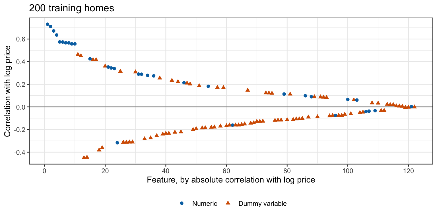
10 features have a correlation above 0.5 in absolute value, led by Gr_Liv_Area, Total_Bsmt_SF, and First_Flr_SF, and 73 of the 122 are below 0.2. Some features nearly repeat others, such as Garage_Cars and Garage_Area (correlation 0.90), but the principal components of the standardized features spread their variance widely: the first 17 explain half of it, and 59 are needed for 90%.
26.2.2 Six fits
Each method is fit by a function that takes the features and responses of a set of homes and returns original-scale estimates for every value of its tuning parameter, one column per value:
- Least squares on all \(p\) features, with no tuning parameter.
- Forward stepwise selection,
leaps::regsubsets(method = "forward")as in the Subset Selection lecture, for every size \(d = 0, 1, \ldots, p\). - Ridge regression, minimizing \(RSS + \lambda\sum_{j=1}^p\beta_j^2\) on the standardized features, from the closed form of the ridge lecture computed by the singular value decomposition, on a grid of \(\lambda\).
- The lasso, minimizing \(RSS + \lambda\sum_{j=1}^p\left|\beta_j\right|\), by
glmnet()with \(\lambda_{\text{glmnet}} = \lambda/(2n)\) as in the Lasso lecture, on a grid of \(\lambda\). - PCR on the first \(M\) principal components of the standardized features, and PLS on the first \(M\) PLS directions, computed as in the PCR and PLS lecture, for \(M = 1, \ldots, p\).
The standardized features are
\[\tilde x_{ij} = \frac{x_{ij} - \bar x_j}{s_j},\]
where
- \(\bar x_j\) and \(s_j\) are the mean and standard deviation (divisor \(n\)) of feature \(j\) over the homes the method is fit to, and
- \(\tilde{\mathbf{X}}\) is the \(n \times p\) matrix of the \(\tilde x_{ij}\).
Least squares and forward stepwise selection give the same fits with or without standardization.
Forward stepwise selection is tuned by cross-validation, like the other methods with a tuning parameter, rather than by BIC: the BIC of the Subset Selection lecture fixes \(\sigma^2\) at the estimate from the model with all \(p\) features, which here rests on only \(n - p - 1 = 77\) residual degrees of freedom.
NoteCode
# Standard deviation with divisor n.
sd_n <- function(v) {
  deviations <- v - mean(v)
  sqrt(mean(deviations^2))
}

# Standardized columns of X, with their centers and scales; a constant
# column keeps scale 1, so it stays a column of zeros.
standardize <- function(X) {
  x_center <- colMeans(X)
  x_scale <- apply(X, 2, sd_n)
  x_scale[x_scale < 1e-12] <- 1
  X_centered <- sweep(X, 2, x_center)
  X_std <- sweep(X_centered, 2, x_scale, "/")
  list(X = X_std, center = x_center, scale = x_scale)
}

# Original-scale estimates, intercept first, one column per value of the
# tuning parameter, from standardized-scale estimates B_std.
original_scale <- function(B_std, s, y_bar) {
  b <- B_std / s$scale
  intercept <- y_bar - colSums(b * s$center)
  rbind(`(Intercept)` = intercept, b)
}

# Ridge estimates for each lambda from the singular value decomposition of
# the standardized features; a singular value of 0 contributes nothing, so
# lambda = 0 is least squares with a constant column's estimate 0.
ridge_estimates <- function(X, y, lambdas) {
  s <- standardize(X)
  sv <- svd(s$X)
  positive <- sv$d > 1e-8 * max(sv$d)
  shrink <- outer(sv$d, lambdas, \(d, l) d / (d^2 + l))
  shrink[!positive, ] <- 0
  u_y <- drop(crossprod(sv$u, y - mean(y)))
  B_std <- sv$v %*% (shrink * u_y)
  original_scale(B_std, s, mean(y))
}

# Grids of lambda, largest first.
ridge_grid <- 10^seq(4, -2, length.out = 61)
lasso_grid <- 10^seq(3, -1.5, length.out = 46)

# Least squares, and ridge regression on its grid.
ls_path <- function(X, y) {
  ridge_estimates(X, y, 0)
}
ridge_path <- function(X, y) {
  ridge_estimates(X, y, ridge_grid)
}

# The lasso on its grid by glmnet(), with this chapter's lambda converted,
# a tolerance tight enough to meet the lasso conditions (checked below), and
# every lambda of the grid fit.
lasso_thresh <- 1e-12
lasso_path <- function(X, y, thresh = lasso_thresh) {
  fit <- glmnet(X, y, alpha = 1, lambda = lasso_grid / (2 * length(y)),
                thresh = thresh, maxit = 1e7)
  stopifnot(length(fit$lambda) == length(lasso_grid))
  as.matrix(coef(fit))
}

# Forward stepwise selection for d = 0, ..., p. Columns that are constant or
# collinear in these homes are left out of the search and keep estimate 0;
# sizes beyond the last one reached repeat it.
forward_path <- function(X, y) {
  qr_X <- qr(cbind(1, X), tol = 1e-7)
  usable <- sort(qr_X$pivot[seq_len(qr_X$rank)])[-1] - 1
  fit <- regsubsets(x = X[, usable, drop = FALSE], y = y,
                    method = "forward", nvmax = length(usable))

  # One column per size; size 0 is the null model.
  B <- matrix(0, ncol(X) + 1, ncol(X) + 1,
              dimnames = list(c("(Intercept)", colnames(X)), NULL))
  B[1, 1] <- mean(y)
  estimates <- coef(fit, id = seq_along(usable))
  for (d in seq_along(estimates)) {
    B[names(estimates[[d]]), d + 1] <- estimates[[d]]
  }
  last <- length(usable) + 1
  B[, seq(last, ncol(X) + 1)] <- B[, last]
  B
}

# PCR for M = 1, ..., p: the estimate on component m is the simple
# regression estimate on its scores, u_m' y / d_m.
pcr_path <- function(X, y) {
  s <- standardize(X)
  sv <- svd(s$X)
  positive <- sv$d > 1e-8 * max(sv$d)
  theta <- drop(crossprod(sv$u, y - mean(y))) / sv$d
  theta[!positive] <- 0
  terms <- sweep(sv$v, 2, theta, "*")
  B_std <- t(apply(terms, 1, cumsum))
  original_scale(B_std, s, mean(y))
}

# PLS for M = 1, ..., p by the PCR and PLS lecture's steps: each direction is
# proportional to the covariances of the residual features with the
# response, and the features are replaced by their residuals from its
# scores. The vectors r_m with scores X_std r_m are W (P'W)^{-1}.
pls_path <- function(X, y) {
  s <- standardize(X)
  X_m <- s$X
  y_centered <- y - mean(y)
  W <- matrix(0, ncol(X), ncol(X))
  P <- W
  Z <- matrix(0, nrow(X), ncol(X))
  theta <- numeric(ncol(X))
  first_size <- NA

  for (m in seq_len(ncol(X))) {
    # Direction, stopping once the residual features no longer covary with
    # the response.
    g <- drop(crossprod(X_m, y_centered))
    size <- sqrt(sum(g^2))
    first_size <- if (m == 1) size else first_size
    if (size < 1e-10 * first_size) {
      break
    }
    W[, m] <- g / size

    # Scores, their simple regression estimate, and the residual features.
    Z[, m] <- drop(X_m %*% W[, m])
    zz <- sum(Z[, m]^2)
    theta[m] <- sum(Z[, m] * y_centered) / zz
    P[, m] <- drop(crossprod(X_m, Z[, m])) / zz
    X_m <- X_m - Z[, m] %o% P[, m]
  }

  # Vectors r_m, checked against the scores, and the estimates for every M.
  M_last <- sum(theta != 0)
  kept <- seq_len(M_last)
  R_dir <- W[, kept] %*% solve(crossprod(P[, kept], W[, kept]))
  stopifnot(max(abs(s$X %*% R_dir - Z[, kept])) < 1e-6)
  terms <- sweep(R_dir, 2, theta[kept], "*")
  B_std <- t(apply(terms, 1, cumsum))
  B_std <- B_std[, c(kept, rep(M_last, ncol(X) - M_last)), drop = FALSE]
  original_scale(B_std, s, mean(y))
}

# All six, in the order of the chapter.
method_names <- c("Least squares", "Forward stepwise", "Ridge", "Lasso",
                  "PCR", "PLS")
paths <- setNames(list(ls_path, forward_path, ridge_path, lasso_path,
                       pcr_path, pls_path),
                  method_names)

# The method names as they read inside a sentence, and at its start.
prose_names <- setNames(c("least squares", "forward stepwise selection",
                          "ridge regression", "the lasso", "PCR", "PLS"),
                        method_names)
upper_first <- function(x) {
  paste0(toupper(substr(x, 1, 1)), substr(x, 2, nchar(x)))
}
Each tuning parameter is chosen by 10-fold cross-validation on the training homes, with the folds fold_id drawn with the split. In each fold every method is fit to the training folds only, so the standardization, the forward stepwise path, the principal components, and the PLS directions are all recomputed there, and the held-out fold is predicted with those fits.
NoteCode
# Mean squared error of predictions y_hat of responses y.
mse <- function(y, y_hat) {
  mean((y - y_hat)^2)
}

# Sums of squared errors of held-out fold l, for every value of the tuning
# parameter, from the estimates that path() computes from the training folds.
fold_sse <- function(l, path, X, y, folds) {
  out <- folds == l
  B <- path(X[!out, , drop = FALSE], y[!out])
  y_hat <- cbind(1, X[out, , drop = FALSE]) %*% B
  colSums((y[out] - y_hat)^2)
}

# Cross-validation estimate for every value of the tuning parameter.
cv_estimate <- function(path, X, y, folds) {
  fold_values <- sort(unique(folds))
  sse <- map(fold_values, \(l) fold_sse(l, path, X, y, folds))
  rowSums(do.call(cbind, sse)) / length(y)
}

# Cross-validation of each method on the training homes.
cv_curves <- map(paths, \(path) {
  cv_estimate(path, X_train, y_train, fold_id)
})

# The value of each tuning parameter with the smallest estimate, as a
# column index: forward column 1 is d = 0, and PCR and PLS column m is M = m.
k_chosen <- map_int(cv_curves, which.min)
d_chosen <- k_chosen[["Forward stepwise"]] - 1
lambda_ridge <- ridge_grid[k_chosen[["Ridge"]]]
lambda_lasso <- lasso_grid[k_chosen[["Lasso"]]]
M_pcr <- k_chosen[["PCR"]]
M_pls <- k_chosen[["PLS"]]
cv_min <- map2_dbl(cv_curves, k_chosen, \(cv, k) cv[k])
cv_ls <- cv_min[["Least squares"]]
glmnet() updates one estimate at a time and stops when no update in a pass changes the criterion by more than a tolerance, its argument thresh, times the criterion of the null model. The High Dimensions lecture found that the default stops far from the minimum when the features are near copies of one another, so the fits here are checked against the lasso conditions of that lecture,
\[\tilde{\mathbf{x}}_{\cdot j}^\top r = \frac{\lambda}{2}\,\text{sign}\left(\hat\beta^L_{\lambda j}\right) \quad \text{if } \hat\beta^L_{\lambda j} \ne 0, \qquad \left|\tilde{\mathbf{x}}_{\cdot j}^\top r\right| \le \frac{\lambda}{2} \quad \text{if } \hat\beta^L_{\lambda j} = 0,\]
where
- \(\hat\beta^L_{\lambda j}\) is the lasso estimate of the standardized-scale coefficient of feature \(j\),
- \(\tilde{\mathbf{x}}_{\cdot j}\) is the \(n\)-vector of standardized feature \(j\) over the training homes, and
- \(r\) is the \(n\)-vector of the lasso residuals.
NoteCode
# Standardized training features and centered responses.
s_train <- standardize(X_train)
y_centered <- y_train - mean(y_train)

# Largest failure of the lasso conditions over the grid, relative to
# lambda / 2, for glmnet() with tolerance thresh.
condition_gap <- function(thresh) {
  B <- lasso_path(X_train, y_train, thresh = thresh)
  B_std <- B[-1, ] * s_train$scale
  gaps <- map_dbl(seq_along(lasso_grid), \(k) {
    b <- B_std[, k]
    half <- lasso_grid[k] / 2
    gradient <- drop(crossprod(s_train$X, y_centered - s_train$X %*% b))
    nonzero <- b != 0
    on_set <- abs(gradient[nonzero] - half * sign(b[nonzero]))
    off_set <- pmax(abs(gradient[!nonzero]) - half, 0)
    max(c(on_set, off_set, 0)) / half
  })
  c(largest = max(gaps), at_chosen = gaps[k_chosen[["Lasso"]]])
}
default_thresh <- formals(glmnet)$thresh
gap_default <- condition_gap(default_thresh)
gap_tight <- condition_gap(lasso_thresh)

# A power of 10 as R writes it, such as 1e-07, for prose.
power_text <- function(x) {
  sprintf("1e%d", round(log10(x)))
}
With the default thresh = 1e-7, the fits on the training homes miss the lasso conditions by up to 98% of \(\lambda/2\), at the smallest values of \(\lambda\) on the grid. With thresh = 1e-12, used throughout, they miss by at most 0.28%, and by 0.003% at the chosen \(\lambda\). The check covers the fit to the training homes only; the same tolerance is used, without a separate check, for every fold and every repeated training sample below. Ridge regression needs no such check: its closed form is exact.
Forward stepwise selection fits \(1 + p(p + 1)/2\) least squares models per path, 7,504 for \(p = 122\), and cross-validation repeats the path in each of the 10 folds.
26.2.3 Cross-validation curves
NoteCode
# Log-scale axis of a cross-validation estimate, shared by the three tabs:
# major lines at 0.02, 0.03, 0.04 and 0.05, and limits from the smallest
# estimate of any method to the largest of PCR and PLS, which rise above the
# least squares line; the forward stepwise, ridge and lasso curves that go
# higher are clipped.
cv_axis <- scale_y_log10(breaks = c(0.02, 0.03, 0.04, 0.05),
                         minor_breaks = NULL)
cv_ylim <- c(min(unlist(cv_curves)),
             max(cv_ls, unlist(cv_curves[c("PCR", "PLS")])))

# Axis of lambda over both grids: major lines at powers of 10, minor lines
# midway between them in log space.
lambda_powers <- -2:4
lambda_axis <- scale_x_log10(breaks = 10^lambda_powers,
                             minor_breaks = 10^(lambda_powers + 0.5),
                             labels = scales::label_log())

# The curves of the given methods against their tuning values x, one line
# per method, least squares dashed and each chosen value circled, on a
# log-scale estimate.
curve_plot <- function(methods, x_values) {
  curves <- map(methods, \(m) {
    tibble(method = m, x = x_values[[m]], cv = cv_curves[[m]])
  }) |>
    list_rbind() |>
    mutate(method = factor(method, levels = methods))
  chosen <- curves |>
    group_by(method) |>
    slice_min(cv, n = 1, with_ties = FALSE)
  ggplot(curves, aes(x = x, y = cv, color = method, linetype = method)) +
    geom_hline(yintercept = cv_ls, linetype = "dashed") +
    geom_line() +
    geom_point(data = chosen, size = 4, shape = 1, show.legend = FALSE) +
    cv_axis +
    coord_cartesian(ylim = cv_ylim) +
    scale_color_manual(values = okabe_ito[c(4, 5)]) +
    labs(y = paste0(n_folds, "-fold CV estimate (log scale)"),
         color = NULL, linetype = NULL, title = title_train,
         caption = paste("Dashed line: least squares.",
                         "Circles: the chosen value of each method.")) +
    theme(legend.position = "inside",
          legend.position.inside = c(0.99, 0.03),
          legend.justification = c(1, 0),
          legend.background = element_rect(color = "grey50"))
}

# The tuning values of each method's curve.
x_values <- list(`Forward stepwise` = 0:p, Ridge = ridge_grid,
                 Lasso = lasso_grid, PCR = seq_len(p), PLS = seq_len(p))

# Forward stepwise against d, ridge and lasso against lambda, PCR and PLS
# against M.
forward_plot <- curve_plot("Forward stepwise", x_values) +
  count_axis +
  labs(x = "Number of features d") +
  theme(legend.position = "none")
penalty_plot <- curve_plot(c("Ridge", "Lasso"), x_values) +
  lambda_axis +
  labs(x = expression(lambda ~ "(log scale)"))
direction_plot <- curve_plot(c("PCR", "PLS"), x_values) +
  count_axis +
  labs(x = "Number of components or directions M")

# Line up the panels of the three tabs: the lambda axis uses expressions, whose
# labels are taller than the plain labels of the other two axes.
cv_aligned <- patchwork::align_patches(forward_plot,
                                       penalty_plot,
                                       direction_plot)
forward_tab <- cv_aligned[[1]]
penalty_tab <- cv_aligned[[2]]
direction_tab <- cv_aligned[[3]]

# The tuning values at which a curve is within near_share of its own
# minimum: how many, and the smallest and largest.
near_share <- 0.05
near_min <- function(method) {
  cv <- cv_curves[[method]]
  near <- x_values[[method]][cv < (1 + near_share) * min(cv)]
  c(count = length(near), low = min(near), high = max(near))
}
forward_near <- near_min("Forward stepwise")
pcr_near <- near_min("PCR")

# How far below least squares the lasso curve ends, at the smallest lambda,
# and the values of M at which the PLS curve is above least squares.
lasso_end_gap <- 1 - tail(cv_curves[["Lasso"]], 1) / cv_ls
below_p <- seq_len(p - 1)
pls_cv <- cv_curves[["PLS"]][below_p]
pls_above <- below_p[pls_cv > cv_ls]
pls_excess <- max(pls_cv) / cv_ls - 1
The tabs plot each method’s cross-validation estimate against its tuning parameter, with least squares as a dashed line and each chosen value circled. Forward stepwise selection with \(d = p\), ridge regression and the lasso as \(\lambda \to 0\), and PCR and PLS with \(M = p\) are all least squares.
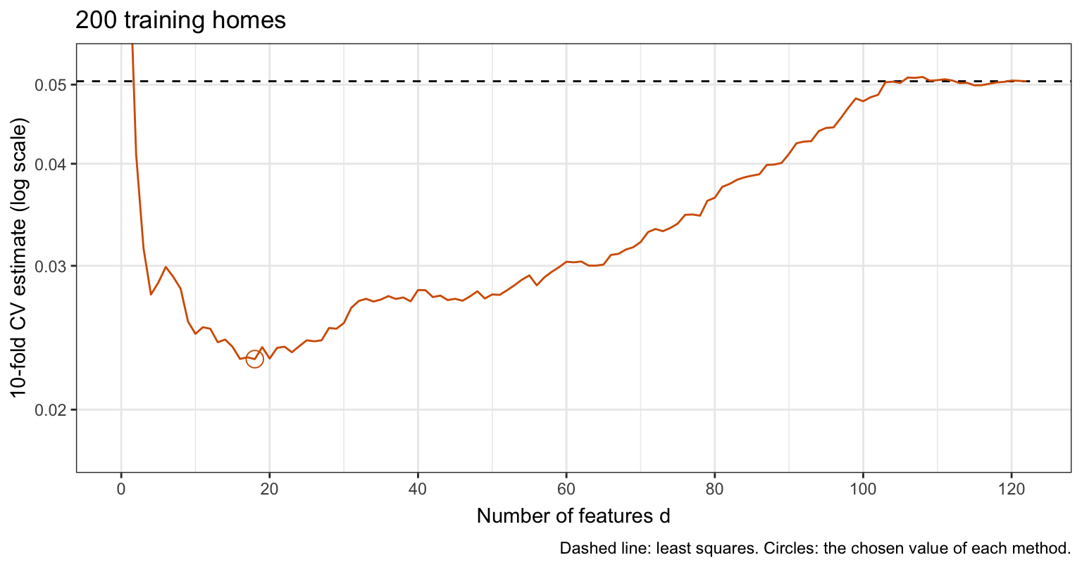
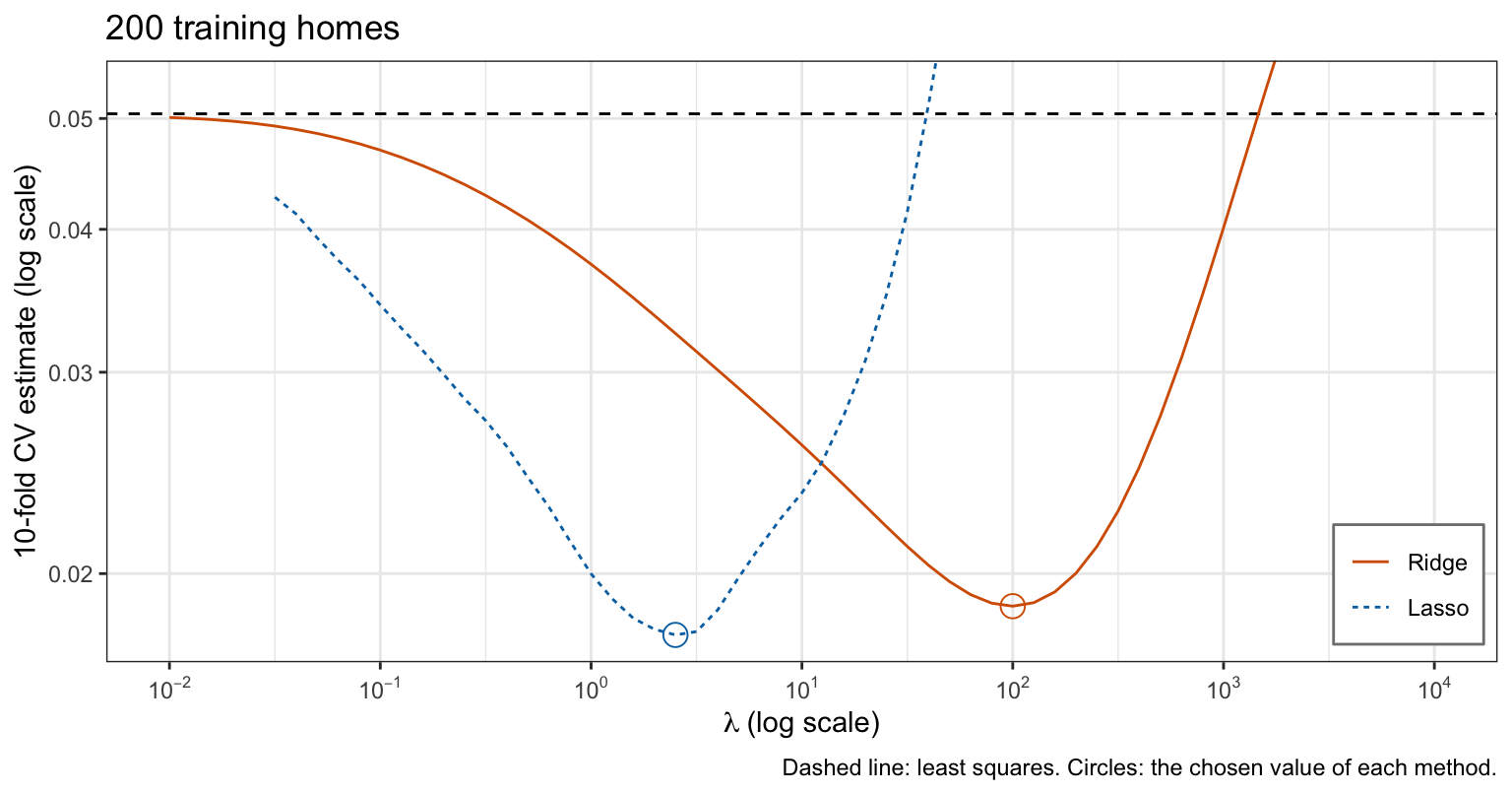
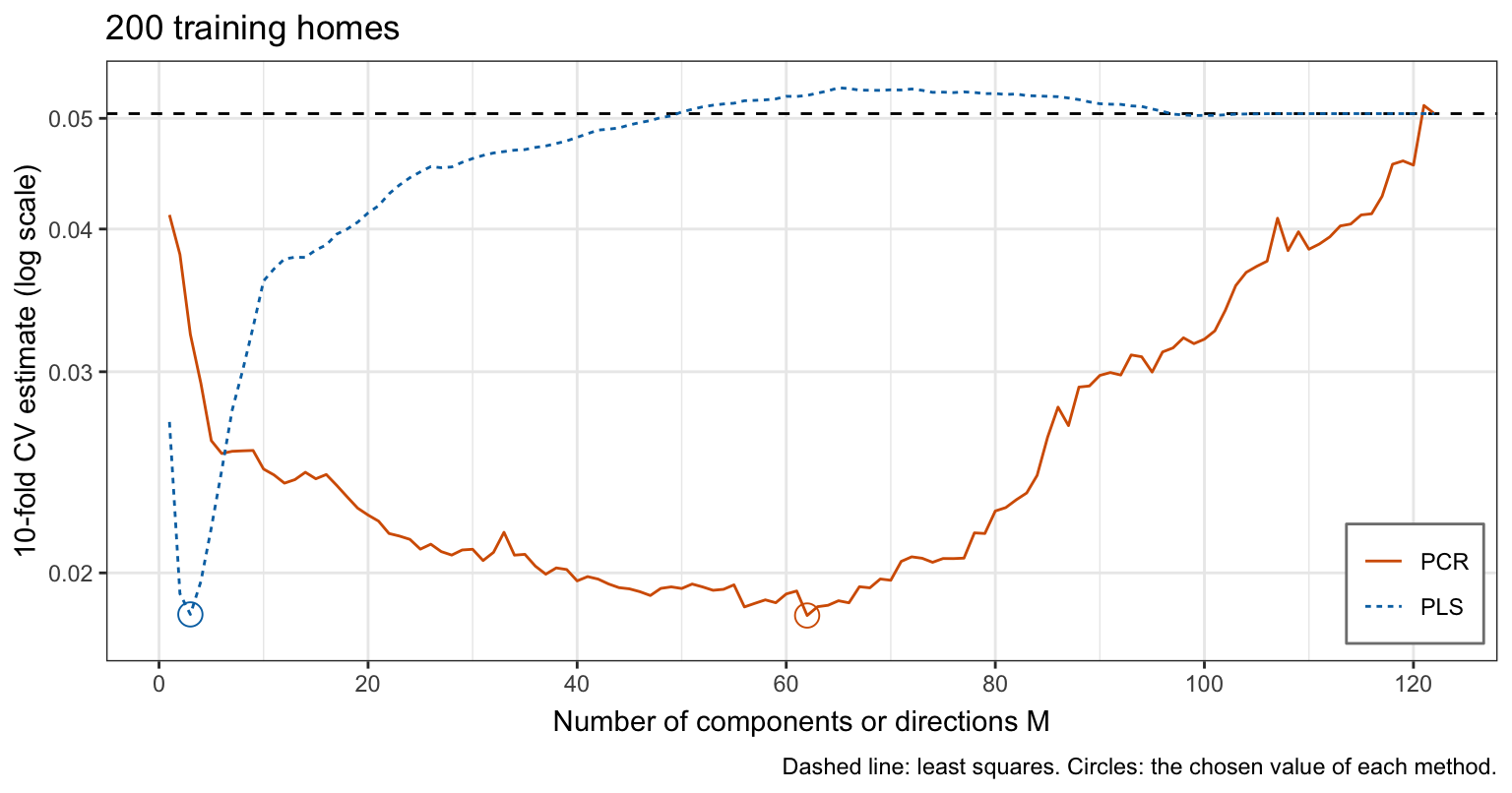
Every curve has its minimum well below the estimate for least squares, 0.0505. Toward the flexible end the forward stepwise and ridge curves rise to the least squares line. The lasso grid stops at \(\lambda = 0.032\), where its curve is still 15% below the line, and the PLS curve rises above the line, by at most 5.4%, at 56 values of \(M\) between 50 and 121, before meeting it at \(M = p\).
- Forward stepwise selection chooses \(d = 18\) features, but its curve is flat: it is within 5% of its minimum at 11 sizes between \(d = 13\) and
- Ridge regression chooses \(\lambda = 100.0\) and the lasso \(\lambda = 2.51\). The two \(\lambda\) are on different scales, one charging squared estimates and the other absolute values, so they are not comparable with each other.
- PLS chooses \(M = 3\) directions and PCR \(M = 62\) components. PLS reaches its minimum with a few directions chosen with the response. PCR’s components are ordered by the variance of the features, not by their relation to price, and its curve is within 5% of its minimum at 12 values of \(M\) between 46 and 66.
26.2.4 Test evaluation
Each method with its chosen tuning parameter is refit to all 200 training homes and evaluated once on the 2,725 test homes.
NoteCode
# Each method refit to the training homes at its chosen value.
chosen_estimates <- map2(paths, k_chosen, \(path, k) {
  path(X_train, y_train)[, k]
})

# Test predictions and test MSE.
test_pred <- map(chosen_estimates, \(b) {
  drop(cbind(1, X_test) %*% b)
})
test_mse <- map_dbl(test_pred, \(y_hat) mse(y_test, y_hat))

# Number of nonzero estimates, intercept excluded.
n_kept <- map_int(chosen_estimates, \(b) sum(b[-1] != 0))

# Table of the tuning value, the nonzero estimates, the cross-validation
# estimate, and the test MSE.
tuning_text <- c("None", paste0("$d = ", d_chosen, "$"),
                 paste0("$\\lambda = ", fmt(lambda_ridge, 1), "$"),
                 paste0("$\\lambda = ", fmt(lambda_lasso, 2), "$"),
                 paste0("$M = ", c(M_pcr, M_pls), "$"))
test_tibble <- tibble(Method = method_names, tuning = tuning_text,
                      kept = n_kept, cv = fmt(cv_min, 4),
                      test = fmt(test_mse, 4))
test_columns <- c("Method", "Tuning", "Nonzero estimates",
                  paste0(n_folds, "-fold CV estimate"), "Test MSE")
test_table <- knitr::kable(test_tibble, col.names = test_columns,
                           align = "llrrr")

# The methods ordered by test MSE, and the relative error in price of a
# root mean squared error on the log scale.
test_order <- names(sort(test_mse))
rmse_factor <- exp(sqrt(test_mse)) - 1

# Cross-validation estimate over test MSE.
cv_over_test <- cv_min / test_mse
tuned <- setdiff(method_names, "Least squares")

# Each chosen fit refit to the training folds of each fold, at the same
# tuning value, and its test MSE averaged over the folds: the effect of
# fitting to fewer homes.
fold_test_mse <- map2_dbl(paths, k_chosen, \(path, k) {
  fold_mses <- map_dbl(seq_len(n_folds), \(l) {
    in_fit <- fold_id != l
    b <- path(X_train[in_fit, ], y_train[in_fit])[, k]
    mse(y_test, cbind(1, X_test) %*% b)
  })
  mean(fold_mses)
})
fold_change <- fold_test_mse / test_mse - 1
n_fold_fit <- n_train - n_train / n_folds| Method | Tuning | Nonzero estimates | 10-fold CV estimate | Test MSE |
|---|---|---|---|---|
| Least squares | None | 122 | 0.0505 | 0.0462 |
| Forward stepwise | \(d = 18\) | 18 | 0.0231 | 0.0269 |
| Ridge | \(\lambda = 100.0\) | 122 | 0.0187 | 0.0241 |
| Lasso | \(\lambda = 2.51\) | 57 | 0.0177 | 0.0228 |
| PCR | \(M = 62\) | 122 | 0.0184 | 0.0262 |
| PLS | \(M = 3\) | 122 | 0.0184 | 0.0246 |
On this training sample the lasso has the smallest test MSE, 0.0228, followed in order by ridge regression, PLS, PCR, forward stepwise selection, and least squares, whose test MSE is 0.0462. A test MSE of 0.0228 is a root mean squared error of 0.151 on the log scale, a typical error of about 16% in price.
The cross-validation estimates of the five tuned methods are 0.70 to 0.86 times their test MSEs, and that of least squares, the one estimate that involves no choice, is 1.09 times its test MSE. Each fold fits 180 homes rather than 200. Refit to the training folds of each fold, least squares has an average test MSE of 0.0590, against 0.0462 for the fit to all 200 homes: with \(p + 1 = 123\) coefficients its residual degrees of freedom fall from \(n - p - 1 = 77\) to 57, and with so few left over its error on new homes rises steeply as homes are removed. For the tuned methods the same refits raise the test MSE by 1.0% to 8.5%, so fewer homes per fold cannot explain why their estimates sit below the test MSE. Each tuned estimate is the smallest on its curve, chosen for being low, and so optimistic, as the Cross-Validation in Practice lecture showed; and all of them rest on the held-out folds of one sample of 200 homes, which may be easier or harder to predict than the test homes.
NoteCode
# The categorical variable of each dummy column.
dummy_columns <- colnames(X_train)[is_dummy]
dummy_variable <- map_chr(dummy_columns, \(column) {
  matches <- categorical[str_starts(column, categorical)]
  matches[which.max(nchar(matches))]
})

# For one method: the number of dummies of each categorical variable, the
# number it keeps, and the variables with some but not all kept.
dummies_kept <- function(method) {
  b <- chosen_estimates[[method]][dummy_columns]
  by_variable <- tibble(variable = dummy_variable, kept = b != 0) |>
    group_by(variable) |>
    summarize(kept = sum(kept), total = n())
  partial <- filter(by_variable, kept > 0, kept < total)
  list(hood = filter(by_variable, variable == "Neighborhood"),
       n_partial = nrow(partial))
}
lasso_dummies <- dummies_kept("Lasso")
forward_dummies <- dummies_kept("Forward stepwise")
hood_reference <- kept_levels(train$Neighborhood, min_homes)[1]
The lasso keeps 57 of the 122 features and forward stepwise selection 18. Neither treats the dummy variables of one categorical explanatory variable as a group. Of the 15 neighborhood dummies, the lasso keeps 8 and forward stepwise selection 3. The lasso keeps some but not all of the dummies of 15 categorical variables, and forward stepwise selection of 4. As in the Subset Selection lecture, a dropped dummy merges its level into the reference: the lasso fit predicts a home in a neighborhood whose dummy it dropped as it predicts an otherwise identical home in North_Ames, the reference. Ridge regression, PCR, and PLS give every dummy a nonzero estimate.
26.3 Repeated training samples
# Number of repeated training samples, and number of test homes at which
# every prediction is made.
n_samples <- 200
n_predict <- 1000
The ranking above belongs to one training sample of 200 homes. As in the ridge and lasso lectures, 1,000 of the 2,725 test homes are the test homes at which every prediction is made, and the remaining 1,725 test homes are the homes from which the repeated training samples are drawn: 200 samples of \(n = 200\) of the remaining test homes. In each sample the candidate features are rebuilt by the three rules from that sample’s homes, every method’s tuning parameter is chosen by 10-fold cross-validation on the sample’s own random folds, and each chosen fit is refit to the sample and predicts the 1,000 test homes.
NoteCode
# Divide the test homes: those at which every prediction is made, and the
# remaining test homes, from which the training samples are drawn.
predict_rows <- sample(n_test, n_predict)
predict_homes <- test[predict_rows, ]
remaining <- test[-predict_rows, ]
y_predict <- predict_homes$log_price
sample_ids <- map(seq_len(n_samples), \(s) sample(nrow(remaining), n_train))

# The whole procedure on one training sample: features, folds,
# cross-validation of every method, refit, and the MSE at the test homes.
fit_sample <- function(id) {
  # Features of the sample and of the test homes, and the sample's folds.
  sample_homes <- remaining[id, ]
  f <- make_features(sample_homes, predict_homes, min_homes)
  y <- sample_homes$log_price
  folds <- sample(rep(seq_len(n_folds), length.out = length(y)))

  # Each method tuned, refit, and evaluated.
  map(method_names, \(method) {
    path <- paths[[method]]
    cv <- cv_estimate(path, f$X, y, folds)
    k <- which.min(cv)
    b <- path(f$X, y)[, k]
    y_hat <- drop(cbind(1, f$X_new) %*% b)
    tibble(method = method,
           p = ncol(f$X),
           k = k,
           kept = sum(b[-1] != 0),
           cv = cv[k],
           test = mse(y_predict, y_hat))
  }) |>
    list_rbind()
}

# Every sample, one row per sample and method.
reps <- map(sample_ids, fit_sample) |>
  list_rbind(names_to = "sample")
reps <- mutate(reps, method = factor(method, levels = method_names))
The samples overlap, since all 200 are drawn from the same 1,725 homes.
26.3.1 Method ranking
NoteCode
# Each method's test MSE relative to the best of the six in the same sample,
# whether it is the best, its rank, and its change from least squares.
reps <- reps |>
  group_by(sample) |>
  mutate(ratio_best = test / min(test),
         won = test == min(test),
         rank = rank(test),
         change_ls = test / test[method == "Least squares"] - 1) |>
  ungroup()

# Summary over the samples, including the median of the chosen fit's
# cross-validation estimate over its test MSE.
rep_summary <- reps |>
  group_by(method) |>
  summarize(mean_test = mean(test), median_test = median(test),
            won = sum(won), median_change = median(change_ls),
            cv_ratio = median(cv / test),
            cv_above = mean(cv > test))
summary_of <- function(methods, column) {
  rep_summary[[column]][match(methods, rep_summary$method)]
}
rep_columns <- c("Method", "Mean test MSE", "Median test MSE",
                 "Samples won", "Median change from least squares")
rep_table <- rep_summary |>
  transmute(Method = method, mean = fmt(mean_test, 4),
            median = fmt(median_test, 4), won = won,
            change = if_else(method == "Least squares", "",
                             pct(median_change, 0))) |>
  knitr::kable(col.names = rep_columns, align = "lrrrr")

# The test MSE relative to the best of the six, one violin per method other
# than least squares, which is far above them, on a log scale.
# Major lines at the round percentages above the best; minor lines midway
# between them in log space.
ratio_percent <- c(0, 5, 10, 25, 50, 100)
ratio_breaks <- 1 + ratio_percent / 100
ratio_labels <- c("Best", paste0("+", ratio_percent[-1], "%"))
ratio_minor <- sqrt(ratio_breaks[-1] * ratio_breaks[-length(ratio_breaks)])
ratio_axis <- scale_y_log10(breaks = ratio_breaks,
                            minor_breaks = ratio_minor,
                            labels = ratio_labels)
rep_plot <- reps |>
  filter(method != "Least squares") |>
  ggplot(aes(x = method, y = ratio_best)) +
  violin +
  ratio_axis +
  labs(x = NULL,
       y = "Test MSE relative to the best\nof the six (log scale)",
       title = paste(n_samples, "training samples of", n_train, "homes"),
       caption = paste("Lines = quartiles and median.",
                       "Least squares, far above, is in the table."))

# Methods by samples won; the most frequent winner, and the methods whose
# test MSE is, in the median sample, within 5% of the winner's.
won_order <- as.character(rep_summary$method[order(-rep_summary$won)])
winners <- won_order[summary_of(won_order, "won") > 0]
non_winners <- setdiff(method_names, winners)
top <- won_order[1]
versus_top <- reps |>
  group_by(sample) |>
  mutate(ratio_top = test / test[method == top]) |>
  group_by(method) |>
  summarize(median_ratio = median(ratio_top),
            beats_top = mean(ratio_top < 1))
close_to_top <- filter(versus_top, method != top,
                       median_ratio < 1 + near_share)
close_names <- prose_names[as.character(close_to_top$method)]

# Share of samples in which the test MSE of method a is below that of b.
beats_share <- function(a, b) {
  test_a <- reps$test[reps$method == a]
  test_b <- reps$test[reps$method == b]
  mean(test_a < test_b)
}

# Every other method against least squares, and forward stepwise selection
# against the four other tuned methods.
beat_ls <- map_dbl(tuned, beats_share, b = "Least squares")
others <- c("Ridge", "Lasso", "PLS", "PCR")
forward_loses <- setNames(map_dbl(others, \(m) {
  beats_share(m, "Forward stepwise")
}), others)
shrink_methods <- c("Ridge", "Lasso", "PLS")

# The rank, in words, of the most frequent winner in the single training
# sample.
rank_words <- c("first", "second", "third", "fourth", "fifth", "sixth")
top_rank_single <- rank_words[match(top, test_order)]
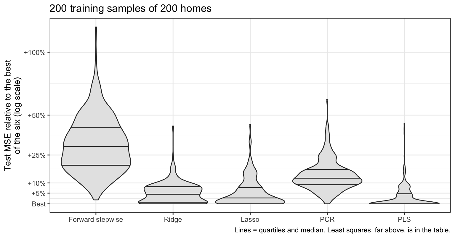
The figure plots, for each sample, the test MSE of each method other than least squares relative to the smallest of the six in that sample. The table summarizes the 200 samples for all six.
| Method | Mean test MSE | Median test MSE | Samples won | Median change from least squares |
|---|---|---|---|---|
| Least squares | 0.0614 | 0.0504 | 0 | |
| Forward stepwise | 0.0303 | 0.0295 | 0 | −42% |
| Ridge | 0.0242 | 0.0240 | 39 | −53% |
| Lasso | 0.0242 | 0.0239 | 52 | −53% |
| PCR | 0.0262 | 0.0258 | 1 | −49% |
| PLS | 0.0237 | 0.0233 | 108 | −54% |
PLS, the lasso, ridge regression, and PCR win 108, 52, 39, and 1 of the 200 samples, and least squares and forward stepwise selection win none. PLS wins most often, but ridge regression and the lasso stay close to it: their test MSEs are a median of 2.3% and 1.6% above that of PLS, and they beat it in 34% and 38% of the samples.
Every other method has a smaller test MSE than least squares in 99.5% to 100.0% of the samples, and improves on it by a median of 42% to 54%. Forward stepwise selection has a larger test MSE than ridge regression, the lasso, and PLS in 98.0% to 99.5% of the samples, and than PCR in 87%.
The single training sample above ranked the lasso first and PLS third. One training sample cannot rank methods whose test MSEs are this close. The large differences, least squares far behind and forward stepwise selection behind ridge regression, the lasso, and PLS, appear in nearly every sample.
Over the samples, the median of the chosen fit’s cross-validation estimate divided by its test MSE is 1.50 for least squares and, for the five tuned methods, forward stepwise selection 0.90, ridge regression 1.02, the lasso 0.98, PCR 0.94, and PLS 1.03. The estimate exceeds the test MSE in 86% of the samples for least squares, for the reason above, and in 34% to 60% for the tuned methods. Their estimates fall on both sides of the test MSE: choosing the smallest estimate pulls them down, fitting each fold to fewer homes pushes them up, and the noise of each sample of 200 homes moves them either way.
26.3.2 Kept features
NoteCode
# Candidate features, forward stepwise size, and nonzero lasso estimates,
# one row per sample.
kept_wide <- reps |>
  filter(method %in% c("Forward stepwise", "Lasso")) |>
  select(sample, p, method, kept) |>
  pivot_wider(names_from = method, values_from = kept)

# The same, one row per sample and count, and their distributions.
count_levels <- c("Candidate features p", "Forward stepwise d",
                  "Lasso nonzero")
kept_counts <- kept_wide |>
  pivot_longer(-sample, names_to = "what", values_to = "count") |>
  mutate(what = factor(what, labels = count_levels,
                       levels = c("p", "Forward stepwise", "Lasso")))

# Number of features: major lines every 25 from 0 to 150, minor lines midway.
kept_axis <- scale_y_continuous(limits = c(0, 150),
                                breaks = seq(0, 150, by = 25),
                                minor_breaks = seq(12.5, 137.5, by = 25))
kept_plot <- ggplot(kept_counts, aes(x = what, y = count)) +
  violin +
  kept_axis +
  labs(x = NULL, y = "Number of features",
       title = paste(n_samples, "training samples of", n_train, "homes"),
       caption = "Lines = quartiles and median.")

# Medians and ranges for prose.
count_stats <- kept_counts |>
  group_by(what) |>
  summarize(median = median(count), low = min(count), high = max(count))
count_of <- function(what, column) {
  count_stats[[column]][count_stats$what == what]
}

# Samples in which the lasso keeps more features than forward stepwise
# selection, as prose.
lasso_more <- mean(kept_wide$Lasso > kept_wide$`Forward stepwise`)
lasso_more_text <- if (lasso_more == 1) {
  "every sample"
} else {
  paste(pct(lasso_more, 1), "of the samples")
}

# Medians of the chosen M of PCR and PLS.
M_median <- reps |>
  filter(method %in% c("PCR", "PLS")) |>
  group_by(method) |>
  summarize(M = median(k)) |>
  deframe()
The figure plots, over the samples, the number of candidate features and the number kept by forward stepwise selection and by the lasso.
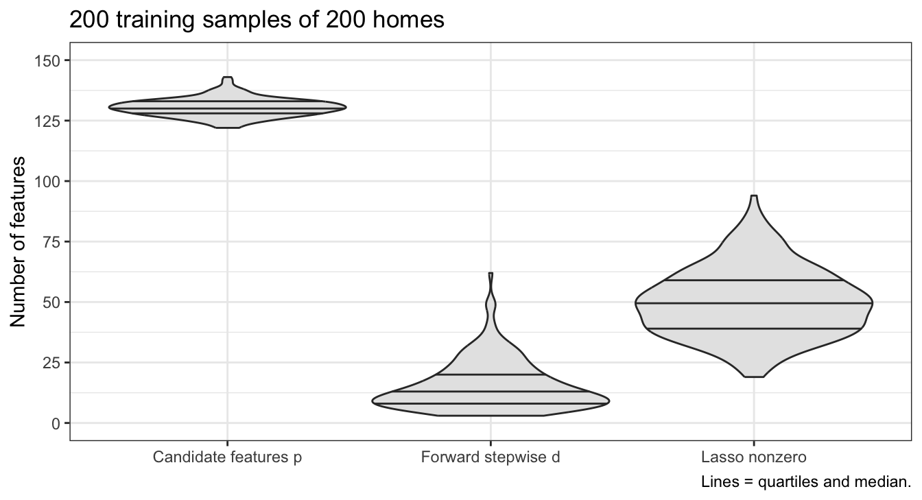
The rules give 122 to 143 candidate features per sample. Forward stepwise selection keeps a median of 13 of them, from 3 to 62, and the lasso a median of 49.5, from 19 to 94. The lasso keeps more features than forward stepwise selection in 99.5% of the samples, each with a shrunken estimate, where forward stepwise selection keeps fewer at their least squares size. Both numbers vary widely from sample to sample, as the lasso’s selected sets did in the Lasso lecture. The median chosen \(M\) is 2 for PLS and 40 for PCR.
26.4 Six methods compared
26.4.1 Properties
NoteCode
# One row per property, one column per method.
properties <- tribble(
  ~Property, ~`Least squares`, ~`Forward stepwise`, ~Ridge, ~Lasso, ~PCR,
  ~PLS,
  "Estimates", "Unconstrained", "Kept: least squares; dropped: 0",
  "All shrunk toward 0, none 0", "Shrunk; some exactly 0",
  "In the span of the first $M$ components", "In the span of $M$ directions",
  "Selects features", "No", "Yes", "No", "Yes", "No", "No",
  "Tuning parameter", "None", "Size $d$", "$\\lambda$", "$\\lambda$", "$M$",
  "$M$",
  "Standardization", "Not needed", "Not needed", "Needed", "Needed",
  "Needed", "Needed",
  "Needs from $n$ and $p$", "$n > p$", "$d < n$", "Any $p$", "Any $p$",
  "$M$ at most the rank of $\\tilde{\\mathbf{X}}$",
  "$M$ at most the rank of $\\tilde{\\mathbf{X}}$",
  "Computation", "One fit", "$1 + p(p + 1)/2$ fits",
  "One SVD for every $\\lambda$", "Coordinate descent for each $\\lambda$",
  "One SVD for every $M$", "One step per direction",
  "Interpretation", "Every estimate", "A least squares model on $d$ features",
  "Every estimate, shrunken", "Some shrunken estimates",
  "Directions; needs every feature", "Directions; needs every feature"
)
properties_table <- knitr::kable(properties, align = "lllllll")
The table collects what the earlier lectures showed about each method; “\(n > p\)” means at least \(p + 1\) observations for the \(p + 1\) coefficients of the model with all \(p\) features, and “\(d < n\)” the same for a model of size \(d\).
| Property | Least squares | Forward stepwise | Ridge | Lasso | PCR | PLS |
|---|---|---|---|---|---|---|
| Estimates | Unconstrained | Kept: least squares; dropped: 0 | All shrunk toward 0, none 0 | Shrunk; some exactly 0 | In the span of the first \(M\) components | In the span of \(M\) directions |
| Selects features | No | Yes | No | Yes | No | No |
| Tuning parameter | None | Size \(d\) | \(\lambda\) | \(\lambda\) | \(M\) | \(M\) |
| Standardization | Not needed | Not needed | Needed | Needed | Needed | Needed |
| Needs from \(n\) and \(p\) | \(n > p\) | \(d < n\) | Any \(p\) | Any \(p\) | \(M\) at most the rank of \(\tilde{\mathbf{X}}\) | \(M\) at most the rank of \(\tilde{\mathbf{X}}\) |
| Computation | One fit | \(1 + p(p + 1)/2\) fits | One SVD for every \(\lambda\) | Coordinate descent for each \(\lambda\) | One SVD for every \(M\) | One step per direction |
| Interpretation | Every estimate | A least squares model on \(d\) features | Every estimate, shrunken | Some shrunken estimates | Directions; needs every feature | Directions; needs every feature |
The methods differ most in what they do to the estimates. Forward stepwise selection applies a hard threshold: a feature is in, at its least squares size given the others, or out at zero. The lasso applies a soft threshold, moving every kept estimate toward zero and setting the rest to zero; for orthogonal features this is the soft thresholding of the lasso lecture. Ridge regression shrinks every estimate and drops none, most strongly along the principal components with the least variance. PCR and PLS replace the \(p\) features by \(M\) directions, keeping each direction’s least squares term in full and dropping the rest, so they select directions, not features.
26.4.2 Expected settings
The earlier lectures suggest a setting in which each method should predict best. These are expectations drawn from their reasoning, some stated here for the first time:
- Least squares when \(n\) is large relative to \(p\): the average variance of its fitted values, \(\sigma^2(p + 1)/n\), is then small, and the Ridge Regression lecture found that shrinkage helped with few training observations per feature and not with more.
- The lasso, and forward stepwise selection, when a few features carry the signal and the rest are noise: the Lasso lecture’s expectation, extended here to forward stepwise selection, which also drops features.
- Ridge regression when many features have small effects of similar size, the contrasting expectation of the lasso lecture.
- PCR when the response is related to the directions in which the features vary most: PCR, like ridge regression, favors those directions, as the PCR and PLS lecture showed.
- PLS when the response is related to other directions: choosing directions with the response can lower the bias of a fit with \(M\) directions, but can add variance.
These are expectations from reasoning, not results. The 2,925 home sales are one dataset, with one structure, and they do not establish any of them: that PLS won most often here, by a few percent, is a finding about these homes and this training sample size, not evidence for or against the expectation for PLS.
NoteBeyond this course
- Other responses. Ridge regression and the lasso extend to logistic and Poisson regression: the penalty is added to the negative log-likelihood in place of the RSS.
glmnet()fits these withfamily = "binomial"orfamily = "poisson". - Elastic net.
glmnet()’salphabetween 0 and 1 mixes the two penalties, keeping some of the lasso’s zeros while shrinking correlated features together as ridge regression does. - Group lasso. Penalizing the length of the vector of a categorical variable’s dummy estimates keeps or drops all of its dummies together.
- Interactions. A penalized fit can include interaction features, with the penalty controlling how many of the many candidate interactions matter.
26.5 Conclusion
Least squares, subset selection, ridge regression, the lasso, PCR, and PLS are six ways of fitting a linear model to the same features, and they differ in what they do to the estimates. Subset selection keeps some features at their least squares estimates and sets the rest to zero, a hard threshold. The lasso shrinks every estimate toward zero and sets some exactly to zero, a soft threshold. Ridge regression shrinks every estimate and sets none to zero. PCR and PLS constrain the estimates to a few directions, chosen without the response for PCR and with it for PLS, and select no feature. Only subset selection and the lasso select features, and both treat each dummy variable of a categorical explanatory variable on its own, so dropping a dummy merges its level into the reference.
Each method other than least squares has one tuning parameter, the size \(d\), the penalty \(\lambda\), or the number of directions \(M\), and each is chosen the same way: by \(k\)-fold cross-validation on the training sample, with the steps of the fit that use the data, the standardization, the forward stepwise path, and the principal components and PLS directions, recomputed from the training folds in each fold. (The rules that defined the candidate features use no responses and were applied once, a simplification.) The chosen fit is refit to all the training data and evaluated once on test data. Its cross-validation estimate can miss its test error in either direction: the smallest estimate on a curve is chosen for being low, so it is optimistic, while fitting each fold to fewer training observations raises it, most for least squares when \(p\) is close to \(n\).
The test MSEs of one training sample rank the methods for that sample only. Comparing them over repeated training samples shows which differences are larger than the variation from sample to sample: how often each method wins and how much it gains over least squares. Each method is expected, from the reasoning of the earlier lectures, to suit a particular setting: least squares when \(n\) is large relative to \(p\), subset selection and the lasso when a few features carry the signal, ridge regression when many features have small effects of similar size, PCR when the response follows the directions in which the features vary most, and PLS when it follows other directions, at a cost in variance. One dataset cannot establish these expectations.
The next class is the review for Exam 2, and Exam 2 follows it. After the exam the course moves to tree-based methods and random forests, ISLR2 Chapter 8.