21 Ridge Regression

Learning objectives

After this lecture you should be able to

write the ridge criterion \(RSS + \lambda\sum_{j=1}^p\beta_j^2\), explain the role of the tuning parameter \(\lambda\) and why the intercept is not penalized, and state the fits it gives as \(\lambda \to 0\) and \(\lambda \to \infty\),
derive the ridge estimate \(\left(\tilde{\mathbf{X}}^\top\tilde{\mathbf{X}} + \lambda\mathbf{I}_p\right)^{-1}\tilde{\mathbf{X}}^\top\left(y - \bar y\mathbf{1}\right)\) for standardized features and a centered response, and derive the mean and variance of the ridge estimator to show that it trades bias for variance,
explain why the features must be standardized before the penalty is applied, although least squares needs no standardization, and why the standardization is repeated inside every cross-validation fold,
explain how the squared bias, the variance, and the test MSE of ridge predictions, defined over repeated training samples, change with \(\lambda\), and why shrinkage helps more when the training sample is small,
choose \(\lambda\) by \(k\)-fold cross-validation on the training data, refit to all the training data, evaluate the chosen model once on test data, and compare it with least squares by test MSE, and
interpret ridge estimates as shrunken but not zero, and explain why the standard errors and \(p\)-values of lm() do not apply to them.

21.1 Delivery times

21.1.1 Data

Question. How long will a food delivery order take, from the time it is placed until it arrives?

Data. modeldata::deliveries records 10,012 delivery orders from one restaurant. The response is time_to_delivery, in minutes. The explanatory variables are the time of day the order was placed (hour, a decimal hour on a 24-hour clock), the day of the week (day), the delivery distance in miles (distance), and 27 columns item_01, item_02, … that count how many of each menu item the order contains.

The test orders are split off first, before any plotting or fitting. The training data are a small random sample of orders; every other order is test data. The next lecture, on the lasso, uses the same split and the same folds.

# The data, the training sample size, and the larger training sample size
# of the bias-variance section.
deliveries <- modeldata::deliveries
n_orders <- nrow(deliveries)
n_train <- 100
n_large <- 300

# Training orders: a random sample; every other order is a test order.
train_id <- sample(n_orders, n_train)
train <- deliveries[train_id, ]
test <- deliveries[-train_id, ]
n_test <- nrow(test)

# Folds for 10-fold cross-validation of the training orders.
n_folds <- 10
fold_labels <- rep(seq_len(n_folds), length.out = n_train)
fold_id <- sample(fold_labels)

These sample() calls are the first random draws after set.seed(20261017). That leaves 100 training orders and 9,912 test orders. The training sample size was chosen to be small relative to the 36 coefficients of the model below, so that their estimates are poorly determined; the bias-variance section also shows what happens with 300 training orders. The tabs plot the delivery time of the training orders against distance, hour, and the total number of items in the order, and against the day.

Code

# The 27 item-count columns.
item_names <- sprintf("item_%02d", 1:27)

# Number of training orders and median delivery time on each day.
day_n <- table(train$day)
day_med <- tapply(train$time_to_delivery, train$day, median)

# Labels shared by the two plots.
title_train <- labs(y = "Delivery time (minutes)",
                    title = paste(n_train, "training orders"))
panel_names <- c(distance = "Distance (miles)",
                 hour = "Hour of order (24-hour clock)",
                 items = "Total number of items")

# Total number of items in each training order.
items_per_order <- rowSums(train[item_names])

# One row per training order and numeric variable.
numeric_long <- train |>
  mutate(items = items_per_order) |>
  pivot_longer(c(distance, hour, items), names_to = "variable") |>
  mutate(variable = factor(panel_names[variable], levels = panel_names))

# Delivery time against distance, hour, and total items.
numeric_plot <- ggplot(numeric_long, aes(x = value, y = time_to_delivery)) +
  geom_point(size = 1) +
  facet_wrap(~ variable, scales = "free_x") +
  labs(x = NULL) +
  title_train

# Delivery time on each day, with the median of each day.
day_labels <- paste0(names(day_n), "\n(", day_n, ")")
day_plot <- ggplot(train, aes(x = day, y = time_to_delivery)) +
  geom_point(position = position_jitter(width = 0.15, height = 0, seed = 1)) +
  stat_summary(fun = median,
               fun.min = median,
               fun.max = median,
               geom = "crossbar",
               width = 0.5,
               color = "#D55E00") +
  scale_x_discrete(labels = day_labels) +
  labs(x = "Day (number of training orders)",
       caption = "Bars = median delivery time.") +
  title_train

# Correlations between the pairs of item counts.
item_cor_matrix <- cor(train[item_names])
item_cors <- item_cor_matrix[upper.tri(item_cor_matrix)]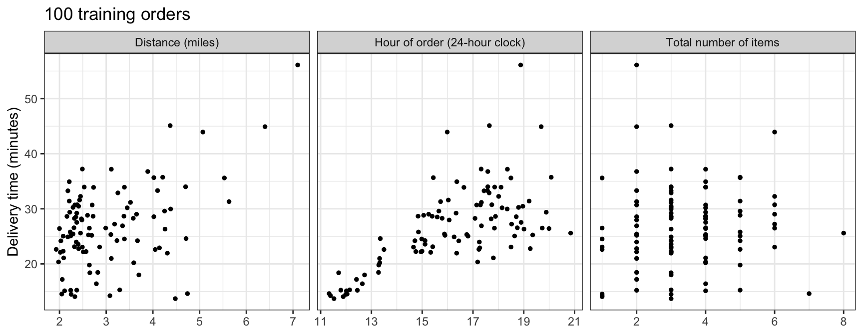

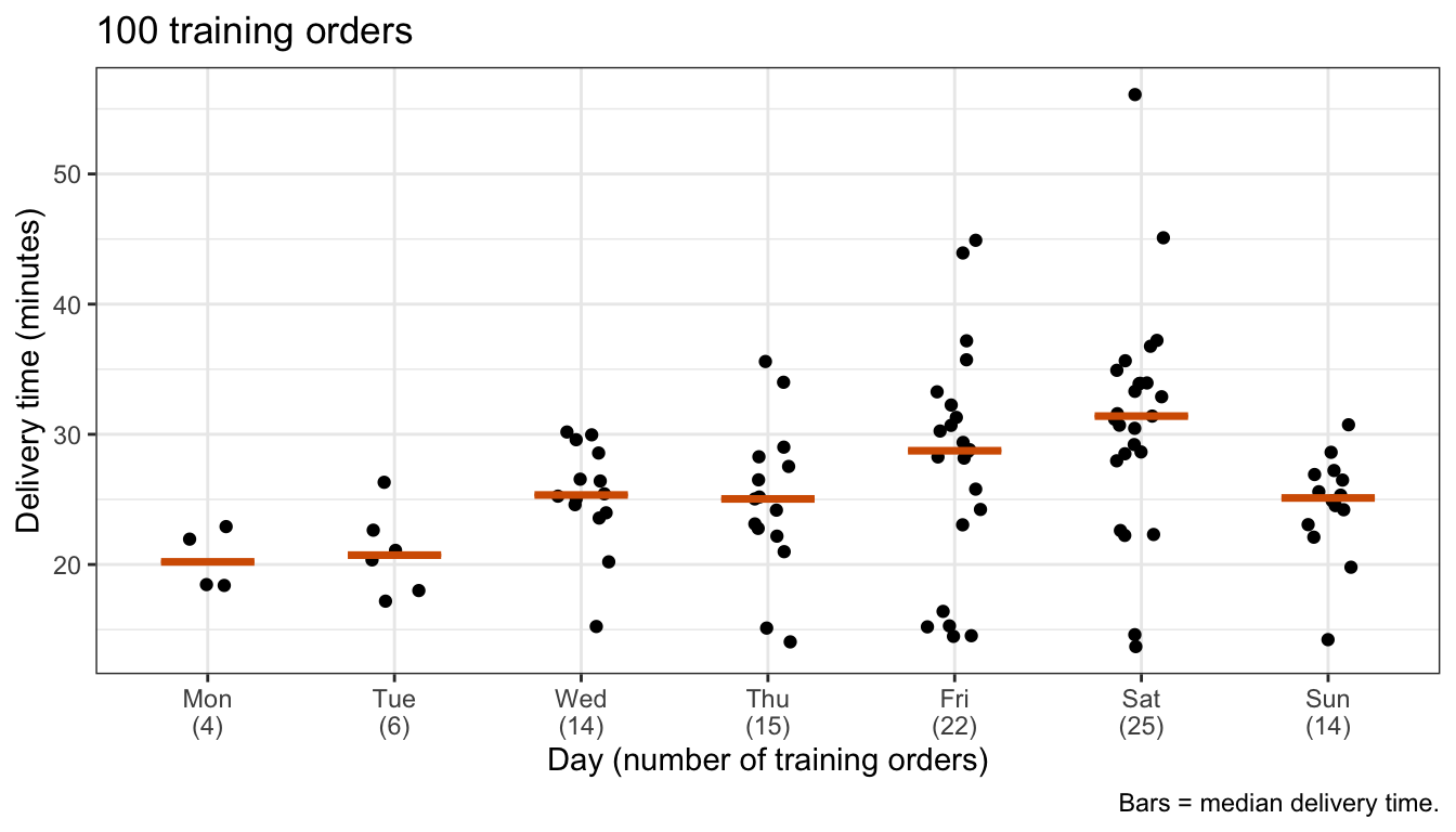
Delivery time rises with distance and with the hour of the order: steeply from 11:00 to about 13:30 and more slowly after, so a straight line in hour is only an approximation. It rises less clearly with the number of items. The median delivery time is shortest on Monday and Tuesday (20.2 and 20.7 minutes), between 25.0 and 25.3 minutes on Wednesday, Thursday, and Sunday, and longest on Friday and Saturday (28.7 and 31.4), but only 4 of the training orders were placed on a Monday and 6 on a Tuesday. The item counts are nearly uncorrelated with each other: over the 351 pairs of items, the median absolute correlation in the training orders is 0.07, and 97% of the pairs are below 0.2 in absolute value.

21.1.2 Features

# The model matrix of a data set, without the column of ones.
model_matrix <- function(data) {
  X <- model.matrix(time_to_delivery ~ ., data = data)
  X[, -1]
}

# Features and responses of the training and test orders.
X_train <- model_matrix(train)
y_train <- train$time_to_delivery
X_test <- model_matrix(test)
y_test <- test$time_to_delivery
p <- ncol(X_train)

hour, distance, and the 27 item counts enter as features as recorded. day enters as 6 dummy variables with Monday as the reference level, so the model has \(p = 35\) features:

\[y_i = \beta_0 + \sum_{j=1}^p \beta_j x_{ij} + \epsilon_i, \qquad \epsilon_i \stackrel{ind}{\sim} N\left(0, \sigma^2\right),\]

where

\(y_i\) is the delivery time of training order \(i = 1, \ldots, n\), with \(n = 100\),
\(x_{ij}\) is the value of feature \(j = 1, \ldots, p\) for order \(i\), in the order hour, dayTue, dayWed, dayThu, dayFri, daySat, daySun, and distance, and the item counts, and \(x_i = \left(1, x_{i1}, \ldots, x_{ip}\right)\) is row \(i\) of the model matrix \(\mathbf{X}\),
\(\beta_0, \ldots, \beta_p\) are the coefficients, and
\(\epsilon_i\) is the error, with variance \(\sigma^2\).

21.1.3 Least squares

Code

# Mean squared error of predictions y_hat of responses y.
mse <- function(y, y_hat) {
  mean((y - y_hat)^2)
}

# Least squares fit to the training orders, and its training and test MSE.
ls_fit <- lm(time_to_delivery ~ ., data = train)
ls_train_mse <- mse(y_train, fitted(ls_fit))
ls_test_pred <- predict(ls_fit, test)
ls_test_mse <- mse(y_test, ls_test_pred)

# Observed and predicted delivery times of the training and test orders.
train_label <- paste(n_train, "training orders")
test_label <- paste(big(n_test), "test orders")
set_labels <- c(train_label, test_label)
ls_train_points <- tibble(set = set_labels[1],
                          observed = y_train,
                          predicted = fitted(ls_fit))
ls_test_points <- tibble(set = set_labels[2],
                         observed = y_test,
                         predicted = ls_test_pred)
ls_points <- bind_rows(ls_train_points, ls_test_points) |>
  mutate(set = factor(set, levels = set_labels))

# Delivery time against prediction, one panel for each set of orders.
ls_plot <- ggplot(ls_points, aes(x = predicted, y = observed)) +
  geom_point(alpha = 0.3, size = 0.8) +
  geom_abline(color = "#D55E00", linewidth = 0.8) +
  facet_wrap(~ set) +
  labs(x = "Least squares prediction (minutes)",
       y = "Delivery time (minutes)",
       title = paste("Least squares with", p,
                     "features, fit to the training orders"),
       caption = "Line: delivery time = prediction.")

The figure plots the delivery time against the least squares prediction, for the training orders the model was fit to and for the test orders.

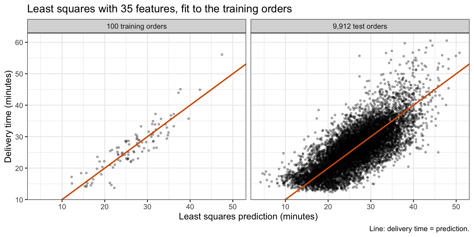
The training orders sit closer to the line than the test orders. The training MSE is 10.13 and the test MSE 22.02, 2.17 times as large. The Subset Selection lecture showed that, for a correct linear model, the training RSS underestimates the error on new responses at the same feature values by \(2(p + 1)\sigma^2\) on average. With \(E\left[RSS\right] = \sigma^2(n - p - 1)\), the fact that makes \(\hat\sigma^2 = RSS/(n - p - 1)\) unbiased, the expected error on those new responses is \(\sigma^2(n + p + 1)\), a ratio of \((n + p + 1)/(n - p - 1) = 2.12\) here, close to the observed ratio, although the test orders have new feature values as well as new responses. With \(p + 1 = 36\) coefficients estimated from 100 orders, the average variance of the fitted values, \(\sigma^2(p + 1)/n\), is 36% of the error variance.

21.2 Ridge regression

The figure counts how many of the 100 training orders contain each menu item.

Code

# Number of training orders containing each item.
orders_with <- colSums(train[item_names] > 0)

# The items as a factor ordered by the number of orders.
item_sorted <- reorder(item_names, orders_with)
item_orders <- tibble(item = item_sorted, orders = orders_with)

# One bar for each item, sorted by the number of orders.
item_count_plot <- ggplot(item_orders, aes(x = orders, y = item)) +
  geom_col(fill = "grey60") +
  labs(x = "Training orders containing the item",
       y = NULL,
       title = paste(n_train, "training orders"))

# The item in the fewest training orders.
rarest <- names(which.min(orders_with))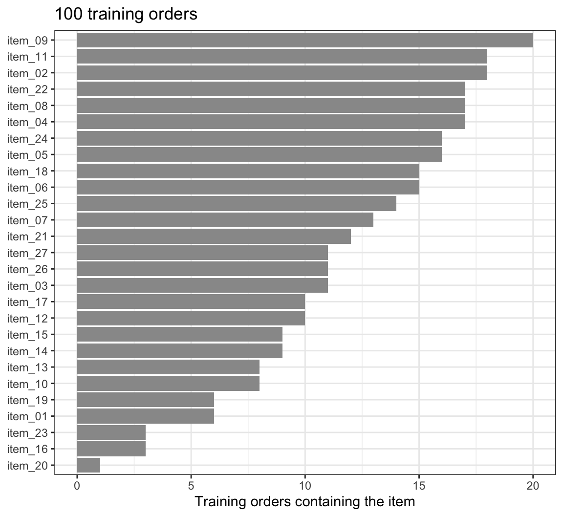

Each item appears in between 1 and 20 of the training orders, a median of 11. item_20 appears in only one order, so its least squares estimate is set almost entirely by how far that order’s delivery time is from the prediction of the other features, its error \(\epsilon_i\) included. Ridge regression keeps every feature but pulls the estimates toward zero.

21.2.1 Penalized criterion

Ridge regression estimates the coefficients by minimizing

\[\sum_{i=1}^n\left(y_i - \beta_0 - \sum_{j=1}^p\beta_j\tilde x_{ij}\right)^2 + \lambda\sum_{j=1}^p\beta_j^2 = RSS + \lambda\sum_{j=1}^p\beta_j^2,\]

where

\(\tilde x_{ij} = \left(x_{ij} - \bar x_j\right)/s_j\) is feature \(j\) of order \(i\) standardized, with \(\bar x_j\) the mean of feature \(j\) over the \(n\) training orders and \(s_j = \sqrt{\frac{1}{n}\sum_{i=1}^n\left(x_{ij} - \bar x_j\right)^2}\) its standard deviation, computed with divisor \(n\),
\(\beta_0\) is the intercept and \(\beta_1, \ldots, \beta_p\) are the coefficients of the standardized features, each the change in mean delivery time per standard deviation of its feature; these are on the standardized scale, where \(\beta_j\) is \(s_j\) times the coefficient of feature \(j\) on the original scale of the model above, and they keep this meaning through the Shrinkage subsection,
\(\lambda \ge 0\) is the tuning parameter, and
\(\lambda\sum_{j=1}^p\beta_j^2\) is the shrinkage penalty.

The RSS rewards values of the coefficients that fit the training orders; the penalty charges \(\lambda\) per unit of squared coefficient, so an estimate grows only as far as the drop in RSS pays for it.

The intercept is not penalized. It is the mean delivery time when every standardized feature is at its mean of zero, and penalizing it would pull every prediction toward zero minutes, an arbitrary point. Without a penalty on \(\beta_0\), adding a constant to every \(y_i\) adds the same constant to the intercept and changes no slope.

21.2.2 Closed form

Write \(\tilde{\mathbf{X}}\) for the \(n \times p\) matrix of standardized features, without a column of ones, \(y\) for the \(n\)-vector of responses, \(\beta = \left(\beta_1, \ldots, \beta_p\right)^\top\), and \(\mathbf{1}\) for the \(n\)-vector of ones. Each column of \(\tilde{\mathbf{X}}\) sums to zero, so \(\mathbf{1}^\top\tilde{\mathbf{X}} = 0\), and the criterion is

\[Q\left(\beta_0, \beta\right) = \left(y - \beta_0\mathbf{1} - \tilde{\mathbf{X}}\beta\right)^\top\left(y - \beta_0\mathbf{1} - \tilde{\mathbf{X}}\beta\right) + \lambda\beta^\top\beta.\]

Setting the derivatives to zero,

\[\frac{\partial Q}{\partial \beta_0} = -2\,\mathbf{1}^\top\left(y - \beta_0\mathbf{1} - \tilde{\mathbf{X}}\beta\right) = -2\left(n\bar y - n\beta_0\right) = 0 \quad\Rightarrow\quad \hat\beta_0 = \bar y,\]

\[\frac{\partial Q}{\partial \beta} = -2\,\tilde{\mathbf{X}}^\top\left(y - \bar y\mathbf{1} - \tilde{\mathbf{X}}\beta\right) + 2\lambda\beta = 0 \quad\Rightarrow\quad \hat\beta^R_\lambda = \left(\tilde{\mathbf{X}}^\top\tilde{\mathbf{X}} + \lambda\mathbf{I}_p\right)^{-1}\tilde{\mathbf{X}}^\top\left(y - \bar y\mathbf{1}\right),\]

where \(\mathbf{I}_p\) is the \(p \times p\) identity matrix, \(\hat\beta_0 = \bar y\) is the standardized-scale intercept, and \(\hat\beta^R_\lambda\) is the ridge estimate of the standardized-scale coefficients for tuning parameter \(\lambda\). \(Q\) is a convex quadratic, so this is its minimum. For \(\lambda > 0\) the matrix \(\tilde{\mathbf{X}}^\top\tilde{\mathbf{X}} + \lambda\mathbf{I}_p\) is invertible even when \(\tilde{\mathbf{X}}^\top\tilde{\mathbf{X}}\) is not, so the ridge estimate is unique even when \(p \ge n\). Two limits bracket every ridge fit:

\(\lambda = 0\): \(\hat\beta^R_0\) is the least squares estimate on the standardized features, which gives the same predictions as least squares on the features as recorded.
\(\lambda \to \infty\): \(\hat\beta^R_\lambda \to 0\), every estimated slope goes to zero, and every prediction is \(\hat\beta_0 = \bar y\), the null model.

An estimate on the original scale is \(\hat\beta^R_{\lambda j}/s_j\), and the original-scale intercept estimate is \(\bar y - \sum_j \bar x_j\hat\beta^R_{\lambda j}/s_j\). The function ridge_fit() computes the closed form and returns the estimates on the original scale.

# Standard deviation with divisor n.
sd_n <- function(v) {
  deviations <- v - mean(v)
  sqrt(mean(deviations^2))
}

# Ridge estimate from the closed form, returned on the original scale.
ridge_fit <- function(X, y, lambda) {
  # Standardize the features.
  center <- colMeans(X)
  scale <- apply(X, 2, sd_n)
  X_centered <- sweep(X, 2, center)
  X_std <- sweep(X_centered, 2, scale, "/")

  # Solve the closed form on the standardized scale.
  lhs <- crossprod(X_std) + lambda * diag(ncol(X))
  rhs <- crossprod(X_std, y - mean(y))
  b_std <- solve(lhs, rhs)

  # Back to the original scale.
  b <- drop(b_std) / scale
  intercept <- mean(y) - sum(b * center)
  c(`(Intercept)` = intercept, b)
}

21.2.3 glmnet scaling

glmnet::glmnet() with alpha = 0 fits ridge regression, but its documented criterion is

\[\frac{1}{2n}RSS + \frac{\lambda_{\text{glmnet}}}{2}\sum_{j=1}^p\beta_j^2,\]

where \(\lambda_{\text{glmnet}}\) is the value glmnet() calls lambda. Multiplying this criterion by \(2n\) gives \(RSS + n\lambda_{\text{glmnet}}\sum_j\beta_j^2\). Two more steps happen inside glmnet() for a numeric response:

it divides \(y\) by its standard deviation \(s_y\) (divisor \(n\)), fits, and multiplies the estimates by \(s_y\) afterward. Fitting \(y/s_y\) with coefficients \(\beta/s_y\) and penalty \(n\lambda_{\text{glmnet}}\) minimizes \(RSS/s_y^2 + n\lambda_{\text{glmnet}}\sum_j\beta_j^2/s_y^2\), the same criterion divided by \(s_y^2\), so this step alone would give \(\lambda = n\lambda_{\text{glmnet}}\);
it also divides the supplied \(\lambda_{\text{glmnet}}\) by \(s_y\) before fitting \(y/s_y\). For the absolute-value penalty of the lasso (next lecture) this division exactly undoes the effect of dividing \(y\) by \(s_y\); glmnet() applies it to the squared penalty too, where it does not.

The net effect, checked numerically below, is that \(\lambda_{\text{glmnet}}\) corresponds to the \(\lambda\) of this chapter’s criterion by

\[\lambda = \frac{n\,\lambda_{\text{glmnet}}}{s_y}.\]

glmnet() standardizes the features itself, with divisor \(n\), and reports estimates on the original scale. The chunk compares it with ridge_fit() at one value of \(\lambda\) on the training orders.

# Standard deviation of the training responses, with divisor n.
s_y <- sd_n(y_train)

# Convert this chapter's lambda to glmnet()'s lambda, and back.
to_glmnet <- function(lambda) {
  lambda * s_y / n_train
}
to_chapter <- function(lambda_glmnet) {
  lambda_glmnet * n_train / s_y
}

# The lambda of the check, and the same lambda on glmnet()'s scale.
lambda_check <- 20
lambda_g <- to_glmnet(lambda_check)

# Check 1: glmnet() at lambda_g against ridge_fit() at lambda_check.
glmnet_check <- glmnet(X_train,
                       y_train,
                       alpha = 0,
                       lambda = lambda_g,
                       thresh = 1e-14)
glmnet_estimates <- coef(glmnet_check)[, 1]
ridge_estimates <- ridge_fit(X_train, y_train, lambda_check)
check_diff <- max(abs(glmnet_estimates - ridge_estimates))

# Check 2: glmnet() on y / s_y, with its estimates multiplied by s_y, against
# ridge_fit() at n * lambda_g, the lambda that dividing y by s_y alone gives.
glmnet_y_std <- glmnet(X_train,
                       y_train / s_y,
                       alpha = 0,
                       lambda = lambda_g,
                       thresh = 1e-14)
y_std_estimates <- s_y * coef(glmnet_y_std)[, 1]
ridge_estimates_n <- ridge_fit(X_train, y_train, n_train * lambda_g)
y_std_diff <- max(abs(y_std_estimates - ridge_estimates_n))

At \(\lambda = 20\) the largest difference between the 36 estimates is \(2.5 \times 10^{-6}\) minutes per unit, within the convergence tolerance of glmnet()’s iterative algorithm. Supplying \(y/s_y\) instead, so that the response glmnet() sees already has standard deviation 1, and multiplying its estimates by \(s_y\) reproduces ridge_fit() at \(\lambda = n\lambda_{\text{glmnet}}\), to within \(2.0 \times 10^{-8}\). From here on \(\lambda\) is this chapter’s, converted where glmnet() is used.

21.2.4 Shrinkage

The closed form, applied to whatever responses a training sample gives, is the ridge estimator: the rule that turns a training sample into an estimate. Bias and variance are properties of the estimator, of how its estimates vary over repeated training samples, not of the estimate from one sample. Treat the features as fixed and suppose the linear model is correct, so \(E\left[y - \bar y\mathbf{1}\right] = \tilde{\mathbf{X}}\beta\) and \(Var\left[y\right] = \sigma^2\mathbf{I}_n\). With \(\mathbf{W}_\lambda = \left(\tilde{\mathbf{X}}^\top\tilde{\mathbf{X}} + \lambda\mathbf{I}_p\right)^{-1}\),

\[E\left[\hat\beta^R_\lambda\right] = \mathbf{W}_\lambda\tilde{\mathbf{X}}^\top\tilde{\mathbf{X}}\beta = \beta - \lambda\mathbf{W}_\lambda\beta, \qquad Var\left[\hat\beta^R_\lambda\right] = \sigma^2\mathbf{W}_\lambda\tilde{\mathbf{X}}^\top\tilde{\mathbf{X}}\mathbf{W}_\lambda.\]

The bias \(-\lambda\mathbf{W}_\lambda\beta\) of the ridge estimator is zero at \(\lambda = 0\) and grows with \(\lambda\). Its variance is smaller than the variance \(\sigma^2\mathbf{A}^{-1}\) of the least squares estimator, where \(\mathbf{A} = \tilde{\mathbf{X}}^\top\tilde{\mathbf{X}}\) is assumed invertible. Take any \(p\)-vector \(a\) and write \(v = \mathbf{W}_\lambda a\), so that \(a = \mathbf{W}_\lambda^{-1}v = \left(\mathbf{A} + \lambda\mathbf{I}_p\right)v\). The linear combination \(a^\top\hat\beta^R_\lambda\) has variance \(\sigma^2a^\top\mathbf{W}_\lambda\mathbf{A}\mathbf{W}_\lambda a = \sigma^2v^\top\mathbf{A}v\), and the least squares \(a^\top\hat\beta\) has variance

\[\sigma^2a^\top\mathbf{A}^{-1}a = \sigma^2v^\top\left(\mathbf{A} + \lambda\mathbf{I}_p\right)\mathbf{A}^{-1}\left(\mathbf{A} + \lambda\mathbf{I}_p\right)v = \sigma^2\left(v^\top\mathbf{A}v + 2\lambda v^\top v + \lambda^2v^\top\mathbf{A}^{-1}v\right).\]

The last two terms are nonnegative for \(\lambda \ge 0\): \(v^\top v\) is a sum of squares, and with \(u = \mathbf{A}^{-1}v\), \(v^\top\mathbf{A}^{-1}v = u^\top\tilde{\mathbf{X}}^\top\tilde{\mathbf{X}}u\) is the sum of squares of \(\tilde{\mathbf{X}}u\). So the ridge estimator of every linear combination of the coefficients, every prediction included, has variance no larger than the least squares estimator’s, and strictly smaller when \(\lambda > 0\) and \(a \ne 0\).

When the standardized features are uncorrelated, as the item counts nearly are, \(\tilde{\mathbf{X}}^\top\tilde{\mathbf{X}} = n\mathbf{I}_p\) and \(\hat\beta^R_{\lambda j} = \frac{n}{n + \lambda}\hat\beta_j\), a fixed fraction of the least squares estimate \(\hat\beta_j\), and the ridge estimator of \(\beta_j\) has mean squared error

\[E\left[\left(\hat\beta^R_{\lambda j} - \beta_j\right)^2\right] = \left(\frac{\lambda}{n + \lambda}\right)^2\beta_j^2 + \left(\frac{n}{n + \lambda}\right)^2\frac{\sigma^2}{n},\]

squared bias plus variance. Summed over \(j\), it is smallest at \(\lambda = p\sigma^2/\sum_j\beta_j^2\), large when the noise is large relative to the coefficients. At that \(\lambda\) the shrinkage factor \(n/(n + \lambda)\) approaches 1 as \(n\) grows, so ridge regression departs most from least squares when the training sample is small.

21.2.5 Standardization

Least squares is scale equivariant: recording distance in feet instead of miles divides its estimate by 5,280 and leaves every prediction unchanged. The figure fits ridge regression to the training orders with centered but unstandardized features, once with distance in miles and once in feet, and with standardized features.

Code

# Grid of lambda values, largest first, used by the later figures too.
lambda_grid <- 10^seq(3, -2, length.out = 101)

# Ridge slopes with centered but unstandardized features.
ridge_raw <- function(X, y, lambda) {
  X_c <- sweep(X, 2, colMeans(X))
  lhs <- crossprod(X_c) + lambda * diag(ncol(X))
  rhs <- crossprod(X_c, y - mean(y))
  drop(solve(lhs, rhs))
}

# The training features with distance in feet.
feet_per_mile <- 5280
X_feet <- X_train
X_feet[, "distance"] <- feet_per_mile * X_feet[, "distance"]

# The distance estimate, in minutes per mile, of the three fits at one lambda.
unit_labels <- c("Unstandardized, miles",
                 "Unstandardized, feet",
                 "Standardized")
scale_rows <- function(lambda) {
  miles <- ridge_raw(X_train, y_train, lambda)[["distance"]]
  feet <- ridge_raw(X_feet, y_train, lambda)[["distance"]]
  standardized <- ridge_fit(X_train, y_train, lambda)[["distance"]]
  tibble(lambda = lambda,
         version = factor(unit_labels, levels = unit_labels),
         distance = c(miles, feet_per_mile * feet, standardized))
}

# The three estimates at every lambda on the grid.
scale_paths <- map(lambda_grid, scale_rows) |>
  list_rbind()

# The k-th of the three estimates at the largest lambda.
at_largest <- scale_paths$lambda == max(lambda_grid)
scale_at <- function(k) {
  scale_paths$distance[at_largest][k]
}

# With standardized features, the distance estimate does not depend on the
# unit.
lambda_unit <- 50
fit_feet <- ridge_fit(X_feet, y_train, lambda_unit)
fit_miles <- ridge_fit(X_train, y_train, lambda_unit)
same_in_feet <- isTRUE(all.equal(feet_per_mile * fit_feet[["distance"]],
                                 fit_miles[["distance"]]))

# The three distance estimates against lambda, least squares in grey.
scale_plot <- ggplot(scale_paths,
                     aes(x = lambda,
                         y = distance,
                         color = version,
                         linetype = version)) +
  geom_hline(yintercept = coef(ls_fit)[["distance"]], color = "grey50") +
  geom_line(linewidth = 0.9) +
  log_lambda +
  scale_color_manual(values = okabe_ito[c(1, 5, 3)]) +
  scale_linetype_manual(values = c("solid", "dashed", "dotdash")) +
  labs(x = expression(lambda ~ "(log scale)"),
       y = "Distance estimate (minutes per mile)",
       color = NULL,
       linetype = NULL,
       title = paste(n_train, "training orders; grey line = least squares")) +
  theme(legend.position = "bottom")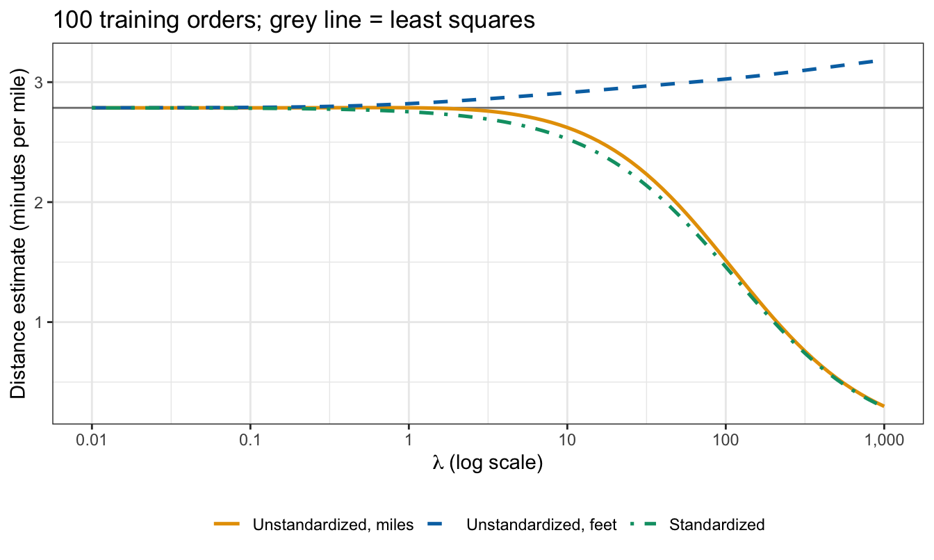

All three agree with least squares as \(\lambda \to 0\). As \(\lambda\) grows the estimate in miles shrinks, to 0.30 minutes per mile at \(\lambda = 1{,}000\). The estimate in feet is never shrunk: it rises to 3.18, above its least squares value of 2.79, as distance takes over part of the effect of the features that are shrunk. With standardized features the fit is the same in either unit: the two distance estimates at \(\lambda = 50\) agree to within the tolerance of all.equal().

So the ridge penalty is not scale equivariant. In feet, the same effect needs a coefficient 5,280 times smaller, whose square the penalty barely charges; without standardization the amount of shrinkage a feature receives depends on its units.

The means \(\bar x_j\) and standard deviations \(s_j\) are computed from the data the model is fit to, so standardization is a data-dependent step. As in the Cross-Validation lecture, it is repeated inside every fold from the training folds only. glmnet() standardizes whatever data it is given, so cv.glmnet() does this automatically.

21.2.6 Estimate path

Code

# Ridge fits to the training orders at every lambda on the grid.
path_fit <- glmnet(X_train,
                   y_train,
                   alpha = 0,
                   lambda = to_glmnet(lambda_grid),
                   thresh = 1e-12)

# Standardized estimates, one column per lambda, smallest lambda first.
x_scale <- apply(X_train, 2, sd_n)
path_coef <- as.matrix(coef(path_fit))
smallest_first <- rev(seq_along(lambda_grid))
path_std <- path_coef[-1, smallest_first] * x_scale

# The four feature groups of the legend.
day_group <- paste0("day (", nlevels(train$day) - 1, " dummies)")
item_group <- paste0("items (", length(item_names), ")")
group_levels <- c("distance", "hour", day_group, item_group)

# The group of each feature name.
feature_group <- function(feature) {
  is_numeric <- feature %in% c("distance", "hour")
  is_day <- str_starts(feature, "day")
  case_when(is_numeric ~ feature,
            is_day ~ day_group,
            TRUE ~ item_group)
}

# One row per feature and lambda, with the group of the feature.
lambda_increasing <- rev(lambda_grid)
path_long <- as_tibble(path_std, rownames = "feature") |>
  pivot_longer(-feature, values_to = "estimate") |>
  mutate(lambda = rep(lambda_increasing, times = p),
         group = feature_group(feature),
         group = factor(group, levels = group_levels))

# Each standardized estimate against lambda.
path_plot <- ggplot(path_long,
                    aes(x = lambda,
                        y = estimate,
                        group = feature,
                        color = group,
                        linetype = group)) +
  geom_hline(yintercept = 0, color = "grey50") +
  geom_line() +
  log_lambda +
  scale_color_manual(values = okabe_ito[c(4, 5, 3, 1)]) +
  scale_linetype_manual(values = c("solid", "longdash", "dotdash", "dotted")) +
  labs(x = expression(lambda ~ "(log scale)"),
       y = "Standardized estimate\n(minutes per standard deviation)",
       color = NULL,
       linetype = NULL,
       title = paste("Ridge estimate path,", n_train, "training orders")) +
  theme(legend.position = "bottom")

# Estimates at the smallest and the largest lambda, the three largest at the
# smallest, and the features whose estimate changes sign.
path_small <- path_std[, 1]
path_large <- path_std[, ncol(path_std)]
small_sorted <- sort(abs(path_small), decreasing = TRUE)
top_std <- names(small_sorted)[1:3]
changed_sign <- names(path_small)[sign(path_small) != sign(path_large)]

# Whether a feature's estimate, along the path, moves away from zero
# somewhere.
moves_away <- function(b) {
  size_change <- diff(abs(b))
  any(size_change > 1e-8)
}

# Number of features whose estimate moves away from zero somewhere.
moving_away <- apply(path_std, 1, moves_away)
not_monotone <- sum(moving_away)

# Length of the vector of standardized estimates at each lambda.
path_length <- sqrt(colSums(path_std^2))
length_falls <- all(diff(path_length) <= 1e-10)

The figure plots each standardized estimate of the ridge fit to the training orders against \(\lambda\), from \(0.01\) to \(1{,}000\).

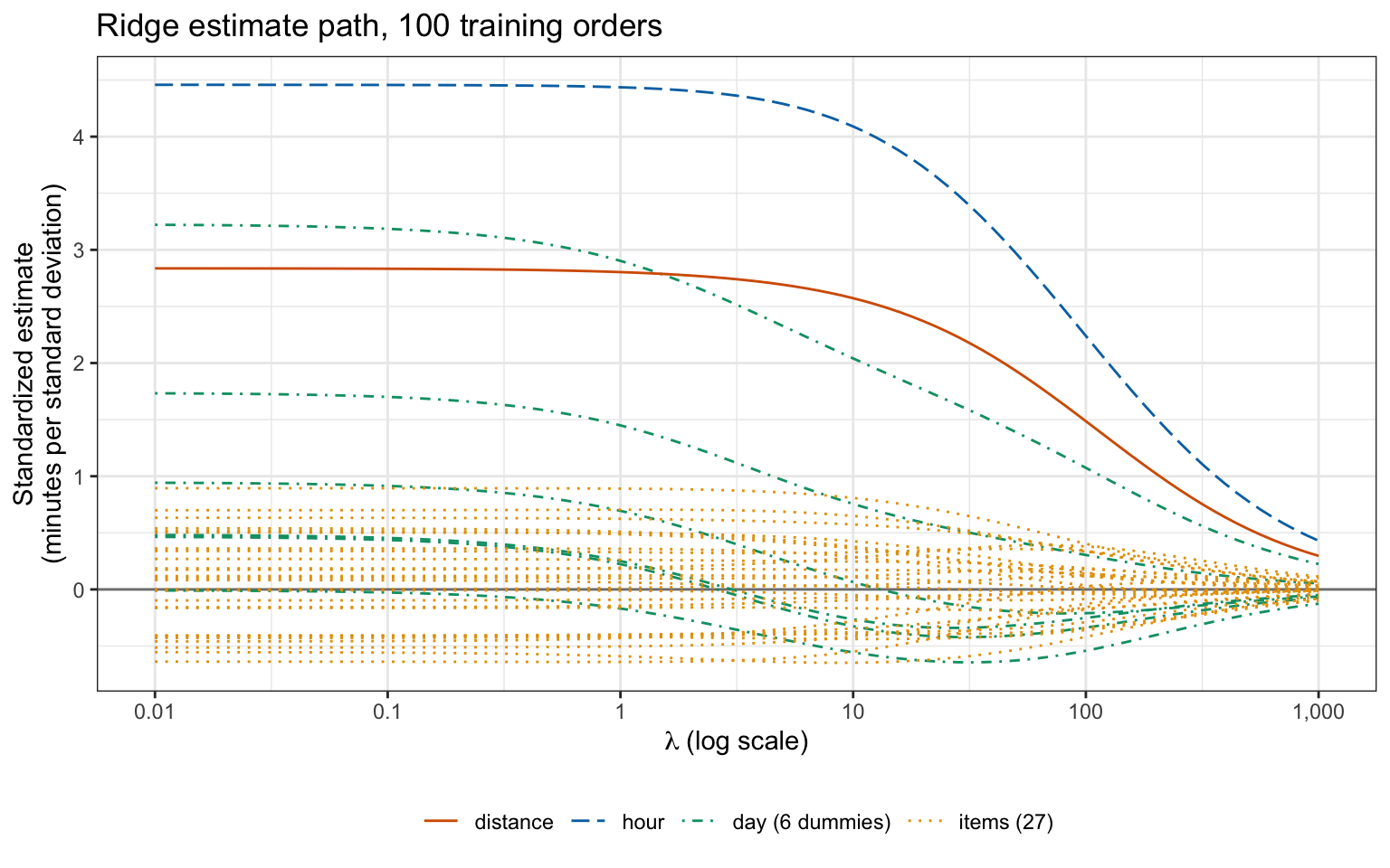
At the left the estimates are those of least squares. The largest are hour (4.5), daySat (3.2), and distance (2.8) minutes per standard deviation, and 31 of the 35 are within a minute of zero. As \(\lambda\) grows the estimates move toward zero smoothly, and none reaches it: at \(\lambda = 1{,}000\) the hour estimate is still 0.43. The length of the vector of standardized estimates falls at every step of the grid, from 6.89 to 0.66, but a single estimate need not: 20 of the 35 move away from zero somewhere along the path, and 8 change sign, among them 3 of the 6 day dummies. The dummy variables of one categorical explanatory variable are correlated, since an order placed on one day was placed on no other, and the penalty shrinks them together.

21.3 Bias-variance tradeoff

Code

# Number of repeated training samples, and number of test orders at which
# every prediction is made.
n_samples <- 500
n_predict <- 4000

# Split the test orders: the test orders at which every prediction is made,
# and the remaining test orders, from which the training samples are drawn.
predict_rows <- sample(n_test, n_predict)
predict_orders <- test[predict_rows, ]
remaining <- test[-predict_rows, ]
n_remaining <- nrow(remaining)
X_predict <- model_matrix(predict_orders)
y_predict <- predict_orders$time_to_delivery
X_remaining <- model_matrix(remaining)
y_remaining <- remaining$time_to_delivery

# f*: least squares fit to the test orders at which predictions are made.
star_fit <- lm(time_to_delivery ~ ., data = predict_orders)
f_star <- fitted(star_fit)
mse_star <- mse(y_predict, f_star)

# The ridge estimate for many lambdas at once, from the singular value
# decomposition of the standardized features. A feature absent from a sample
# gets estimate 0, which at lambda = 0 is least squares on the rest.
ridge_path <- function(X, y, lambdas) {
  # Standardize; a feature constant in the sample is centered only.
  center <- colMeans(X)
  scale <- apply(X, 2, sd_n)
  scale[scale == 0] <- 1
  X_centered <- sweep(X, 2, center)
  X_std <- sweep(X_centered, 2, scale, "/")

  # Shrinkage d / (d^2 + lambda) of each singular value d at each lambda,
  # and 0 for a singular value of 0.
  sv <- svd(X_std)
  shrink <- outer(sv$d,
                  lambdas,
                  \(d, l) ifelse(d > 1e-8, d / (d^2 + l), 0))

  # Standardized estimates, one column per lambda, then the original scale.
  y_centered <- y - mean(y)
  u_y <- drop(crossprod(sv$u, y_centered))
  b_std <- sv$v %*% (shrink * u_y)
  b <- b_std / scale

  # One intercept per lambda, above the slopes.
  intercept <- mean(y) - colSums(b * center)
  rbind(`(Intercept)` = intercept, b)
}

# ridge_path() agrees with ridge_fit().
path_check <- ridge_path(X_train, y_train, 20)[, 1]
fit_check <- ridge_fit(X_train, y_train, 20)
paths_agree <- all.equal(path_check, fit_check, check.attributes = FALSE)
stopifnot(isTRUE(paths_agree))

# Grid of lambda values, and the test orders whose predictions are shown.
bv_lambdas <- c(0, 10^seq(-1, 3, length.out = 41))
show_rows <- 1:8

# Squared bias, variance, and test MSE at the test orders in X_predict, over
# the training samples whose rows of the remaining test orders are in ids.
bias_variance <- function(ids) {
  # Running sums over the samples: one row per test order, one column per
  # lambda.
  sum_pred <- matrix(0, n_predict, length(bv_lambdas))
  sum_sq <- matrix(0, n_predict, length(bv_lambdas))
  sum_err <- matrix(0, n_predict, length(bv_lambdas))
  shown <- list()

  for (id in ids) {
    # Ridge fit to one training sample, predicting the test orders.
    b <- ridge_path(X_remaining[id, ], y_remaining[id], bv_lambdas)
    pred <- cbind(1, X_predict) %*% b

    # Add this sample's predictions to the running sums.
    sum_pred <- sum_pred + pred
    sum_sq <- sum_sq + pred^2
    sum_err <- sum_err + (y_predict - pred)^2
    shown <- c(shown, list(pred[show_rows, ]))
  }

  # Average over the M samples, then over the test orders.
  M <- length(ids)
  f_bar <- sum_pred / M
  curves <- tibble(lambda = bv_lambdas,
                   variance = colMeans(sum_sq / M - f_bar^2),
                   bias2 = colMeans((f_bar - f_star)^2),
                   mse = colMeans(sum_err / M),
                   gap = mse - mse_star - bias2 - variance)
  best <- slice_min(curves, mse, n = 1)
  list(curves = curves, shown = shown, best = best)
}

# Training samples of 100 orders, then of 300, from the remaining test orders.
sample_ids <- map(seq_len(n_samples), \(s) sample(n_remaining, n_train))
bv_100 <- bias_variance(sample_ids)
sample_ids_large <- map(seq_len(n_samples), \(s) sample(n_remaining, n_large))
bv_300 <- bias_variance(sample_ids_large)

# The lambda with the smallest test MSE for training samples of 100.
lambda_sim <- bv_100$best$lambda

# The largest lambda, and the labels of the shown test orders.
lambda_big <- max(bv_lambdas)
order_labels <- paste("Order", show_rows)

# Predictions of the shown test orders at lambda l over the training samples
# of 100, one violin per order, with f* as a cross.
spread_plot <- function(l, label) {
  # Predictions at this lambda, sample after sample.
  col <- which(bv_lambdas == l)
  predictions <- unlist(map(bv_100$shown, \(m) m[, col]))
  order_rep <- rep(order_labels, n_samples)
  spread <- tibble(order = factor(order_rep, levels = order_labels),
                   prediction = predictions)

  # f* at the same orders.
  crosses <- tibble(order = factor(order_labels, levels = order_labels),
                    prediction = f_star[show_rows])

  # Title and caption.
  title <- bquote(.(label) * ", " * .(n_samples) ~ "training samples of" ~
                    .(n_train) ~ "orders")
  caption <- paste("Lines = quartiles and median; cross = least squares",
                   "fit to the", big(n_predict), "test orders.")

  ggplot(spread, aes(x = order, y = prediction)) +
    geom_violin(fill = "grey90",
                scale = "width",
                quantiles = c(0.25, 0.5, 0.75),
                quantile.linetype = "solid") +
    geom_point(data = crosses,
               shape = 4,
               size = 3,
               stroke = 1.3,
               color = "#D55E00") +
    coord_cartesian(ylim = c(10, 45)) +
    labs(x = "Test order",
         y = "Predicted delivery time (minutes)",
         title = title,
         caption = caption)
}

# Least squares, the lambda with the smallest test MSE, and the largest.
lambda_sim_text <- fmt(lambda_sim, 1)
lambda_big_text <- big(lambda_big)
label_mid <- bquote("Ridge, " * lambda == .(lambda_sim_text))
label_big <- bquote("Ridge, " * lambda == .(lambda_big_text))
spread_plots <- list(spread_plot(0, "Least squares"),
                     spread_plot(lambda_sim, label_mid),
                     spread_plot(lambda_big, label_big))

To see what shrinkage does to predictions, this section draws repeated training samples. Of the 9,912 test orders, 4,000 are the test orders at which every prediction is made, and the remaining 5,912 test orders are the orders from which the repeated training samples are drawn. Both sets are part of this chapter’s test orders: the demonstration chooses nothing, and the delivery model is chosen and fit from the 100 training orders alone. From the remaining test orders, 500 training samples of 100 orders were drawn, ridge regression was fit to each sample at each \(\lambda\) on a grid, and each fit predicted the 4,000 test orders. The test MSE in this section’s figures is the mean squared error at those 4,000 test orders, averaged over the samples.

The tabs plot the predictions of 8 of the 4,000 test orders for three values of \(\lambda\). Each violin shows one order’s predictions over the 500 training samples, and the cross marks its fitted value from least squares fit to the 4,000 test orders themselves.

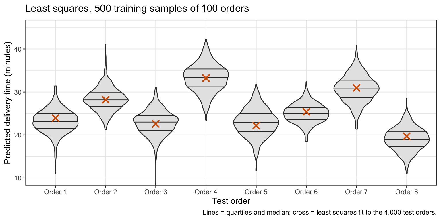
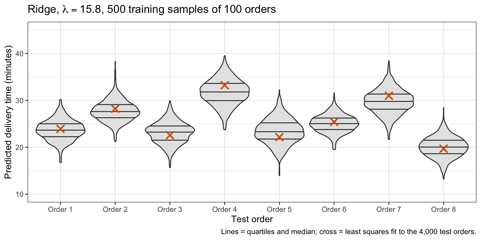
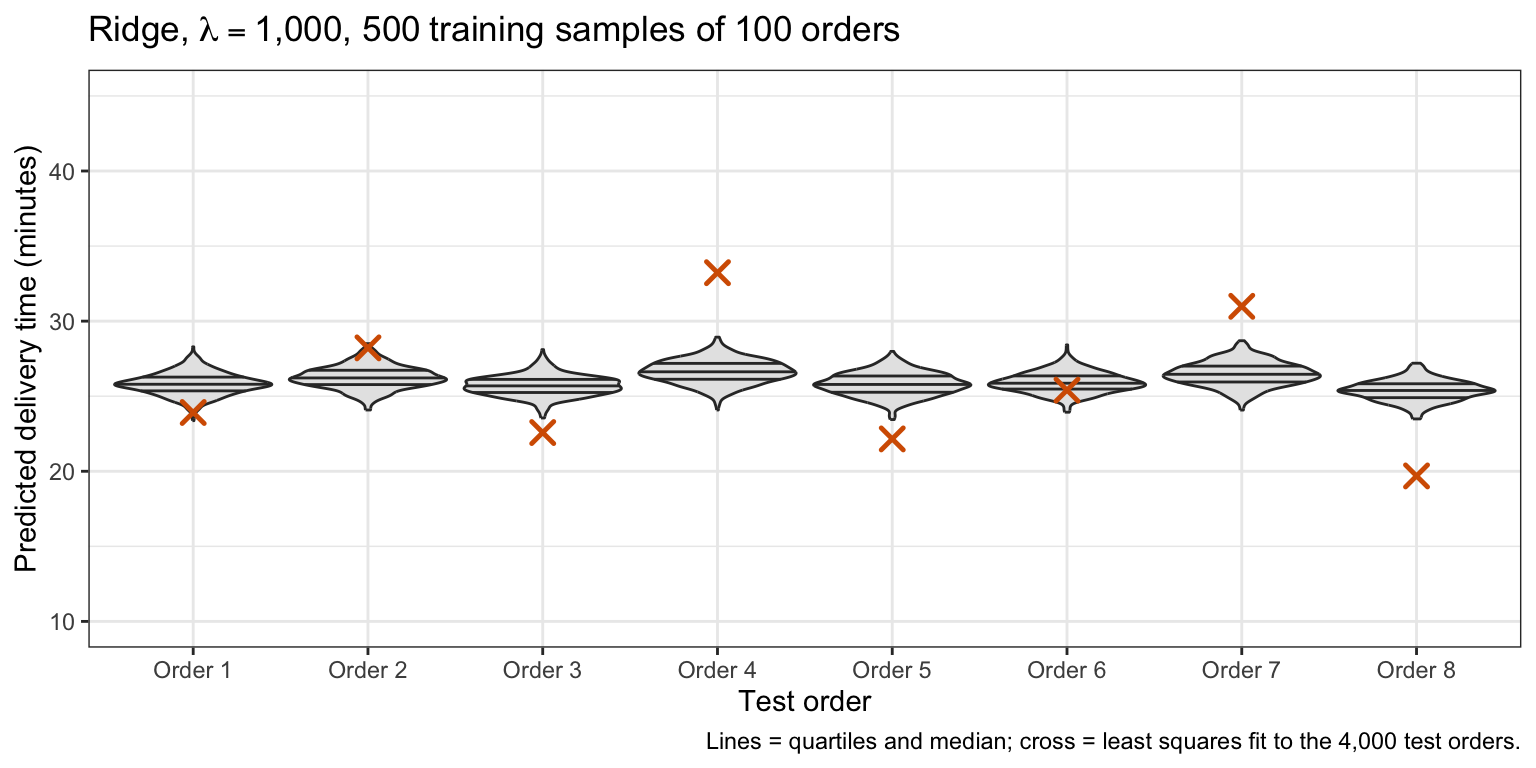
With \(\lambda = 0\), least squares, each order’s predictions are centered near its cross but spread over several minutes. At \(\lambda = 15.8\) they spread less and are pulled slightly toward the mean. At \(\lambda = 1{,}000\) they spread least, but they are pulled toward the mean delivery time, above the cross for the quick orders and below it for the slow ones.

21.3.1 Squared bias and variance

Index the test orders at which predictions are made by \(i \in \mathcal{T}\) and the training samples by \(m = 1, \ldots, M\), and write \(\hat f^{(m)}_\lambda(x_i)\) for the ridge prediction of order \(i\) from sample \(m\). Over the samples,

\[\bar f_\lambda(x_i) = \frac{1}{M}\sum_{m=1}^M\hat f^{(m)}_\lambda(x_i), \qquad \text{Variance}(\lambda) = \frac{1}{|\mathcal{T}|}\sum_{i \in \mathcal{T}}\frac{1}{M}\sum_{m=1}^M\left[\hat f^{(m)}_\lambda(x_i) - \bar f_\lambda(x_i)\right]^2,\]

\[\text{Bias}^2(\lambda) = \frac{1}{|\mathcal{T}|}\sum_{i \in \mathcal{T}}\left[\bar f_\lambda(x_i) - f^*(x_i)\right]^2, \qquad \text{MSE}(\lambda) = \frac{1}{|\mathcal{T}|}\sum_{i \in \mathcal{T}}\frac{1}{M}\sum_{m=1}^M\left[y_i - \hat f^{(m)}_\lambda(x_i)\right]^2,\]

where

\(\mathcal{T}\) is the set of the \(|\mathcal{T}| = 4{,}000\) test orders at which every prediction is made, and \(y_i\) the delivery time of order \(i\),
\(M = 500\) is the number of repeated training samples, each of \(n\) of the 5,912 remaining test orders,
\(\bar f_\lambda(x_i)\) is the average prediction of order \(i\), and
\(f^*(x_i)\) is the fitted value of order \(i\) from least squares fit to the 4,000 test orders in \(\mathcal{T}\), the closest a linear function of these features comes to their delivery times; it explains \(R^2 = 71\%\) of their variability, and it is itself estimated, from 4,000 orders, so even least squares has a small squared bias.

\(\text{Variance}(\lambda)\) measures how much a prediction depends on which orders were sampled, and \(\text{Bias}^2(\lambda)\) how far the average prediction is from \(f^*\). Both are estimates from \(M\) samples. The bias is measured against the best linear function of these features, not against the true mean delivery time, so error from a nonlinear effect of hour, for example, is in neither term. \(\text{MSE}(\lambda)\) is the test MSE.

Expanding the square in \(\text{MSE}(\lambda)\) around \(\bar f_\lambda(x_i)\), the cross term sums to zero over \(m\). Expanding again around \(f^*(x_i)\), the cross term is \(\frac{2}{|\mathcal{T}|}\sum_{i \in \mathcal{T}}\left[y_i - f^*(x_i)\right]\left[f^*(x_i) - \bar f_\lambda(x_i)\right] = 0\): least squares residuals are orthogonal to every linear function of the features, and \(f^*(x_i) - \bar f_\lambda(x_i)\), a difference of averages of linear predictions, is one. So

\[\text{MSE}(\lambda) = \text{MSE}^* + \text{Bias}^2(\lambda) + \text{Variance}(\lambda),\]

where \(\text{MSE}^* = \frac{1}{|\mathcal{T}|}\sum_{i \in \mathcal{T}}\left[y_i - f^*(x_i)\right]^2 = 13.71\) does not depend on \(\lambda\). In the simulation the two sides differ by at most \(1.2 \times 10^{-13}\), rounding error.

21.3.2 Training sample size

Code

# The three curves, in legend order.
term_labels <- c("Variance plus squared bias", "Squared bias", "Variance")

# Upper limit of the vertical axis, the same in both tabs.
y_max <- max(bv_100$curves$variance + bv_100$curves$bias2)

# Squared bias, variance, and their sum against lambda, for training samples
# of n orders; lambda = 0 is drawn as points at 0.03, left of the grid.
bv_plot <- function(bv, n) {
  # One row per lambda and curve.
  curves <- bv$curves |>
    transmute(lambda = if_else(lambda == 0, 0.03, lambda),
              `Variance plus squared bias` = variance + bias2,
              `Squared bias` = bias2,
              Variance = variance) |>
    pivot_longer(-lambda, names_to = "term", values_to = "value") |>
    mutate(term = factor(term, levels = term_labels))
  curves_grid <- filter(curves, lambda > 0.05)
  curves_ls <- filter(curves, lambda < 0.05)

  # Position of the smallest test MSE, and the title.
  best_x <- max(bv$best$lambda, 0.03)
  title <- paste(n_samples, "training samples of", n,
                 "orders; dotted line = smallest test MSE")

  ggplot(curves_grid,
         aes(x = lambda,
             y = value,
             color = term,
             linetype = term,
             shape = term)) +
    geom_line(linewidth = 0.9) +
    geom_point(data = curves_ls, size = 2.5) +
    geom_vline(xintercept = best_x, color = "grey50", linetype = "dotted") +
    scale_x_log10(breaks = c(0.03, 0.1, 1, 10, 100, 1000),
                  labels = c("0", "0.1", "1", "10", "100", "1,000")) +
    scale_color_manual(values = okabe_ito[c(4, 5, 3)]) +
    scale_linetype_manual(values = c("solid", "dashed", "dotdash")) +
    scale_shape_manual(values = c(16, 17, 15)) +
    coord_cartesian(ylim = c(0, y_max)) +
    labs(x = expression(lambda ~ "(log scale; points at the left are" ~
                          lambda == 0 * ")"),
         y = "Minutes squared",
         color = NULL,
         linetype = NULL,
         shape = NULL,
         title = title) +
    theme(legend.position = "bottom")
}
bv_plots <- list(bv_plot(bv_100, n_train), bv_plot(bv_300, n_large))

# Value of one column of the curves at one lambda.
bv_at <- function(bv, l, col) {
  bv$curves[[col]][bv$curves$lambda == l]
}

# Reduction in test MSE at the best lambda, relative to least squares.
gain <- function(bv) {
  1 - bv$best$mse / bv_at(bv, 0, "mse")
}

# The result for training samples of 300, for the prose.
if (bv_300$best$lambda == 0) {
  gain_300_text <- paste("no $\\lambda$ on the grid has a smaller test MSE",
                         "than least squares")
} else {
  gain_300 <- gain(bv_300)
  gain_300_pct <- if (gain_300 < 0.001) "less than 0.1%" else pct(gain_300)
  gain_300_text <- paste0("the smallest test MSE, at $\\lambda = ",
                          fmt(bv_300$best$lambda, 1), "$, is ",
                          gain_300_pct, " below that of least squares")
}

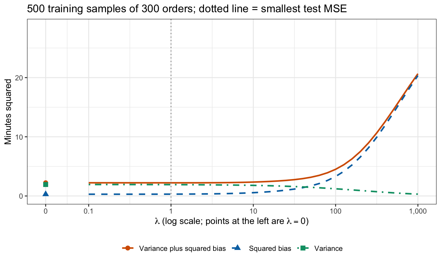
The tabs plot the squared bias, the variance, and their sum against \(\lambda\), from 500 training samples of 100 orders and, separately, 500 of 300 orders. Each sample’s ridge fit at each \(\lambda\) predicts the 4,000 test orders, and each term is averaged over those test orders and over the samples, as defined above. By the identity above, variance plus squared bias is the test MSE minus \(\text{MSE}^*\), which does not depend on \(\lambda\), so it is smallest at the \(\lambda\) with the smallest test MSE, marked by the dotted line.

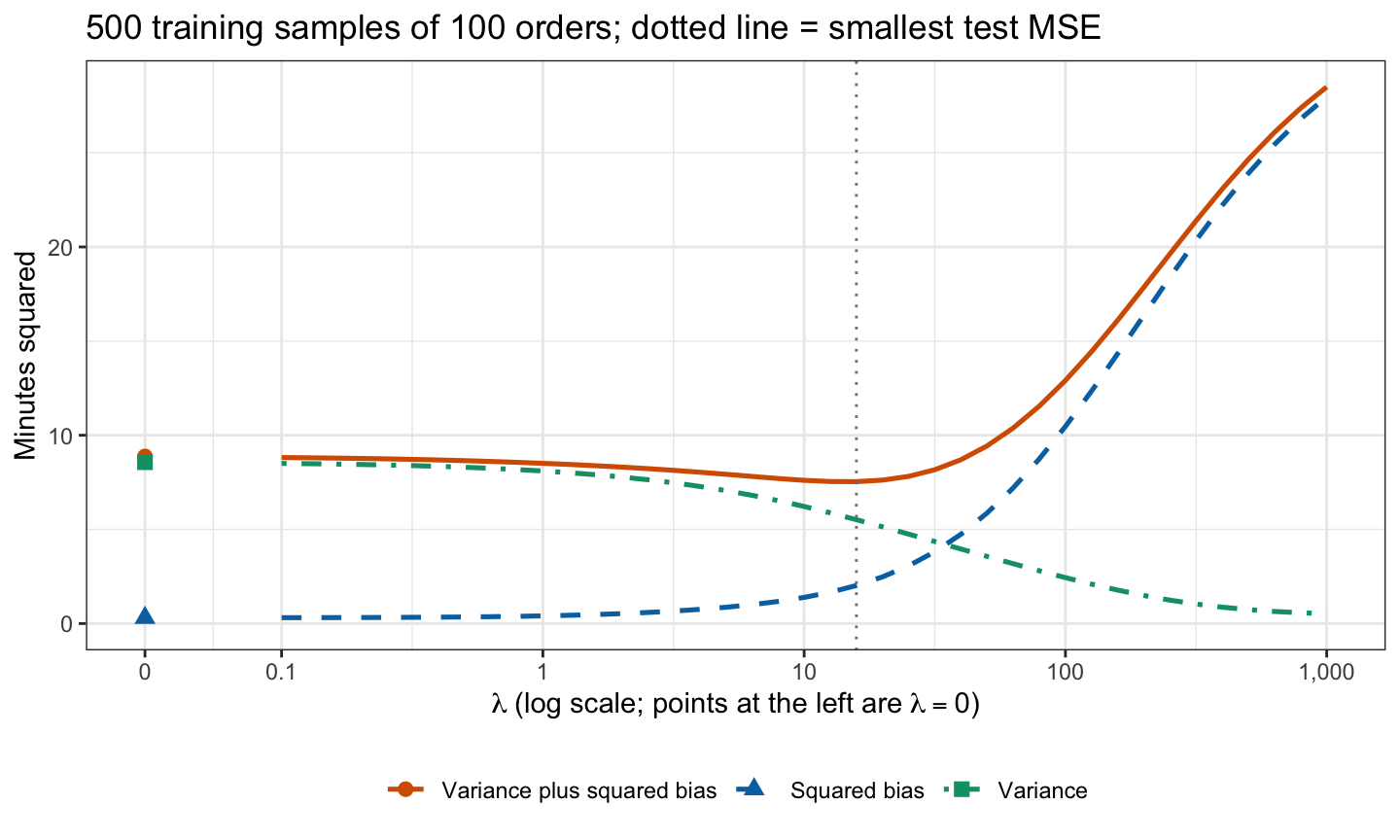
With \(n = 100\), least squares has squared bias 0.30 and variance 8.57. As \(\lambda\) grows the variance falls and the squared bias rises, slowly at first, so their sum falls to its minimum at \(\lambda = 15.8\). There the test MSE is 21.24 against 22.58 for least squares, 5.9% lower. Beyond the minimum the squared bias dominates, and the test MSE climbs toward that of the null model.

With \(n = 300\) the variance of least squares is only 1.94, so there is little for shrinkage to remove before the squared bias from shrinking the large estimates of hour, distance, and the days outweighs it: the smallest test MSE, at \(\lambda = 1.0\), is less than 0.1% below that of least squares. How much shrinkage helps depends on the data and on the sample size, so \(\lambda\) has to be chosen from the training data.

21.4 Tuning parameter selection

21.4.1 Cross-validation

cv.glmnet() computes the \(k\)-fold cross-validation estimate \(\text{CV}_{(k)}(\lambda)\) for every \(\lambda\) on a grid, here the grid of the estimate path converted to glmnet()’s scale, with \(k = 10\) and the folds fold_id drawn with the split. For each fold glmnet() standardizes and fits from the other 9 folds and predicts the held-out fold; the held-out folds are validation sets.

# 10-fold cross-validation on the lambda grid, with the folds of the split.
cv_fit <- cv.glmnet(X_train,
                    y_train,
                    alpha = 0,
                    lambda = to_glmnet(lambda_grid),
                    foldid = fold_id,
                    thresh = 1e-12)

# The lambda with the smallest estimate, on this chapter's scale.
lambda_cv <- to_chapter(cv_fit$lambda.min)

Code

# Least squares on the same folds; ridge_path() at lambda = 0 also handles an
# item absent from the training folds.
ls_mse_in_fold <- function(l) {
  out <- fold_id == l
  b <- ridge_path(X_train[!out, ], y_train[!out], 0)
  pred <- cbind(1, X_train[out, ]) %*% b
  mse(y_train[out], pred)
}
fold_size <- tabulate(fold_id)
ls_fold_mse <- map_dbl(seq_len(n_folds), ls_mse_in_fold)
cv_ls <- weighted.mean(ls_fold_mse, fold_size)

# One standard error over the folds, computed as cv.glmnet() computes it.
ls_fold_var <- weighted.mean((ls_fold_mse - cv_ls)^2, fold_size)
ls_se <- sqrt(ls_fold_var / (n_folds - 1))

# The smallest estimate and its position on the grid.
cv_min <- min(cv_fit$cvm)
i_min <- which.min(cv_fit$cvm)

# Plus or minus one standard error at the minimum and for least squares, the
# range where the two intervals overlap, and its share of each interval.
ridge_interval <- c(cv_fit$cvlo[i_min], cv_fit$cvup[i_min])
ls_interval <- c(cv_ls - ls_se, cv_ls + ls_se)
overlap <- c(max(ridge_interval[1], ls_interval[1]),
             min(ridge_interval[2], ls_interval[2]))
overlap_ridge <- diff(overlap) / diff(ridge_interval)
overlap_ls <- diff(overlap) / diff(ls_interval)

# cv.glmnet() converts with all n training orders, but each fold fit has its
# own n and s_y: the ratio of the lambda a fold applies to the plotted one.
fold_conversion <- function(l) {
  in_fit <- fold_id != l
  sum(in_fit) / sd_n(y_train[in_fit])
}
fold_ratio <- map_dbl(seq_len(n_folds), fold_conversion) / (n_train / s_y)

# Cross-validation with this chapter's lambda applied exactly in every fold.
fold_sse <- function(l) {
  out <- fold_id == l
  b <- ridge_path(X_train[!out, ], y_train[!out], lambda_grid)
  pred <- cbind(1, X_train[out, ]) %*% b
  colSums((y_train[out] - pred)^2)
}
fold_sse_matrix <- sapply(seq_len(n_folds), fold_sse)
cv_exact <- rowSums(fold_sse_matrix) / n_train

# The grid on this chapter's scale; where the estimate rises above least
# squares, and where it is within 1% of its smallest value.
cv_lambda <- to_chapter(cv_fit$lambda)
above_ls <- cv_lambda > lambda_cv & cv_fit$cvm > cv_ls
cv_above_ls <- min(cv_lambda[above_ls])
flat_range <- range(cv_lambda[cv_fit$cvm < 1.01 * cv_min])

# Number of folds in which some item appears in none of the training folds.
item_absent <- function(l) {
  in_fit <- fold_id != l
  any(colSums(X_train[in_fit, ] != 0) == 0)
}
fold_has_absent <- map_lgl(seq_len(n_folds), item_absent)
n_absent_folds <- sum(fold_has_absent)

# The estimate against lambda, least squares as a dashed reference line, and
# the chosen lambda as a point.
cv_curve <- tibble(lambda = cv_lambda, cv = cv_fit$cvm)
ls_label <- "'Least squares, ' * lambda == 0"
chosen_label <- paste0("'Chosen, ' * lambda == ", fmt(lambda_cv, 1))
cv_expand <- expansion(mult = c(0.12, 0.05))
cv_plot <- ggplot(cv_curve, aes(x = lambda, y = cv)) +
  geom_hline(yintercept = cv_ls, linetype = "dashed", color = "#0072B2") +
  geom_line() +
  annotate("point",
           x = lambda_cv,
           y = cv_min,
           size = 3,
           color = "#D55E00") +
  annotate("text",
           x = min(lambda_grid),
           y = cv_ls,
           label = ls_label,
           parse = TRUE,
           vjust = -0.5,
           hjust = 0,
           size = 3.5,
           color = "#0072B2") +
  annotate("text",
           x = lambda_cv,
           y = cv_min,
           label = chosen_label,
           parse = TRUE,
           vjust = 1.8,
           size = 3.5,
           color = "#D55E00") +
  log_lambda +
  scale_y_continuous(breaks = scales::breaks_width(5), expand = cv_expand) +
  labs(x = expression(lambda ~ "(log scale)"),
       y = paste0(n_folds, "-fold CV estimate of test MSE"),
       title = paste(n_train, "training orders"))

The figure plots \(\text{CV}_{(10)}(\lambda)\) against \(\lambda\), with the estimate for least squares on the same folds as a dashed line and the chosen \(\lambda\), the one with the smallest estimate, as a point.

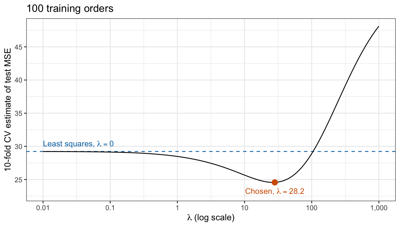
The estimate falls from 29.23 for least squares to its smallest value, 24.57, at \(\lambda = 28.2\) (\(\lambda_{\text{glmnet}} = 2.071\)), and rises again beyond it, above the least squares estimate from \(\lambda = 112\) on.¹ The estimated reduction, 15.9%, is small relative to its uncertainty: plus or minus one standard error is 19.62 to 29.52 at the minimum and 23.51 to 34.95 for least squares. The two intervals overlap from 23.51 to 29.52, 61% of the ridge interval and 53% of the least squares interval. The curve is flat near its minimum: from \(\lambda = 18\) to 35 the estimate is within 1% of its smallest value. In 2 of the 10 folds some item appears in none of the training folds, and glmnet() gives it an estimate of zero. The repeated training samples of the previous section put the smallest average test MSE at \(\lambda = 15.8\); cross-validation sees only the 100 training orders and chooses a larger value.

Beyond this course

One-standard-error rule. cv.glmnet() also reports lambda.1se, the largest \(\lambda\) whose estimate is within one standard error of the smallest, here \(\lambda = 100.0\). It chooses more shrinkage when the curve is flat near its minimum.

21.4.2 Test evaluation

cv.glmnet() also fits the whole path to all 100 training orders, so predicting with s = "lambda.min" uses the model refit to all the training data. The chosen model is evaluated once on test data, the 9,912 test orders, with least squares for comparison.

# Predictions of the model refit to all the training orders at the chosen
# lambda, and its test MSE.
ridge_train_pred <- drop(predict(cv_fit, X_train, s = "lambda.min"))
ridge_test_pred <- drop(predict(cv_fit, X_test, s = "lambda.min"))
ridge_test_mse <- mse(y_test, ridge_test_pred)

Code

# Training MSE, cross-validation estimate, and test MSE of the two fits.
ridge_train_mse <- mse(y_train, ridge_train_pred)
lambda_text <- c("0", fmt(lambda_cv, 1))
train_mses <- c(ls_train_mse, ridge_train_mse)
cv_estimates <- c(cv_ls, cv_min)
test_mses <- c(ls_test_mse, ridge_test_mse)
test_values <- tibble(Method = c("Least squares", "Ridge"),
                      lambda = lambda_text,
                      train = fmt(train_mses),
                      cv = fmt(cv_estimates),
                      test = fmt(test_mses))
test_columns <- c("Method",
                  "$\\lambda$",
                  "Training MSE",
                  paste0(n_folds, "-fold CV estimate"),
                  "Test MSE")
test_table <- knitr::kable(test_values,
                           col.names = test_columns,
                           align = "lrrrr")

# Paired comparison over the test orders.
sq_diff <- (y_test - ls_test_pred)^2 - (y_test - ridge_test_pred)^2
diff_se <- sd(sq_diff) / sqrt(n_test)

# The whole procedure on one repeated training sample: lambda by 10-fold
# cross-validation and a refit, against least squares, both predicting the
# test orders at which every prediction is made.
procedure_one <- function(id) {
  # The training sample, and its own random folds.
  X <- X_remaining[id, ]
  y <- y_remaining[id]
  fold_labels <- rep(seq_len(n_folds), length.out = length(y))
  folds <- sample(fold_labels)

  # Cross-validation, with the grid converted with this sample's n and s_y.
  lambda_sample <- lambda_grid * sd_n(y) / length(y)
  cv_s <- cv.glmnet(X,
                    y,
                    alpha = 0,
                    lambda = lambda_sample,
                    foldid = folds,
                    thresh = 1e-10)

  # Test MSE of least squares and of ridge at the chosen lambda.
  ls_pred <- cbind(1, X_predict) %*% ridge_path(X, y, 0)
  ridge_pred <- predict(cv_s, X_predict, s = "lambda.min")
  tibble(ls = mse(y_predict, ls_pred), ridge = mse(y_predict, ridge_pred))
}
procedure <- function(ids) {
  map(ids, procedure_one) |>
    list_rbind()
}
procedure_100 <- procedure(sample_ids)
procedure_300 <- procedure(sample_ids_large)

# Share of samples in which ridge wins, and its average gain.
win_share <- function(d) {
  mean(d$ridge < d$ls)
}
mean_gain <- function(d) {
  1 - mean(d$ridge) / mean(d$ls)
}

# Gain of this training sample on the test orders, and of every sample of 100.
test_gain <- 1 - ridge_test_mse / ls_test_mse
sample_gain <- 1 - procedure_100$ridge / procedure_100$ls
gain_range <- quantile(sample_gain, c(0.05, 0.95))

Method	\(\lambda\)	Training MSE	10-fold CV estimate	Test MSE
Least squares	0	10.13	29.23	22.02
Ridge	28.2	12.23	24.57	20.38

Ridge regression’s test MSE is 20.38, against 22.02 for least squares, 7.5% lower. The paired difference in squared error over the test orders has mean 1.64 and standard error 0.18, so the improvement is not an accident of which orders are test orders. That standard error treats the two fitted models as fixed: it reflects only which orders are test orders, not which training orders were drawn. Both cross-validation estimates are above the test MSE: each fit in cross-validation uses 90 orders, and with so few orders per feature the error falls quickly as orders are added; an estimate from 100 orders is also noisy. The reduction cross-validation estimated, 15.9%, is 2.1 times the 7.5% reduction on the test orders.

This training sample is a favorable draw. Over the 500 repeated training samples of 100 orders, the same procedure, \(\lambda\) by 10-fold cross-validation and then a refit, has a lower MSE at the 4,000 test orders than least squares in 72% of the samples and a higher one in 28%. Its average MSE is 3.7% below that of least squares; the 7.5% gain on the test orders is 2.0 times as large. The median gain over the samples is 2.9%, 90% of the gains lie between -9.9% and 15.4%, and 25.6% of the samples gain at least as much as this one, which puts it at about the 74th percentile. The average gain is less than the 5.9% of the best fixed \(\lambda\), because cross-validation chooses \(\lambda\) from noisy estimates. With training samples of 300 orders, ridge regression has the lower MSE in only 44% of the samples and a higher one in 56%, and its average MSE is 0.2% above that of least squares. On these data, shrinkage helps modestly with 100 training orders and not at all with 300.

21.5 Ridge estimates

Code

# Estimates of the ridge fit at the chosen lambda and of least squares.
b_ridge <- coef(cv_fit, s = "lambda.min")[, 1]
b_ls <- coef(ls_fit)
feature_order <- colnames(X_train)

# Legend labels.
fit_labels <- c("Least squares", "Ridge")
lambda_cv_text <- fmt(lambda_cv, 1)
ridge_legend <- bquote("Ridge, " * lambda == .(lambda_cv_text))
fit_legend <- c(expression("Least squares"), ridge_legend)

# One row per feature and fit, the features in model order from the top.
feature_rep <- rep(feature_order, 2)
feature_levels <- rev(feature_order)
fit_rep <- rep(fit_labels, each = p)
compare_long <- tibble(
  feature = factor(feature_rep, levels = feature_levels),
  estimate = c(b_ls[feature_order], b_ridge[feature_order]),
  fit = factor(fit_rep, levels = fit_labels)
)

# The two sets of estimates, one row per feature.
coef_compare_plot <- ggplot(compare_long,
                            aes(x = estimate,
                                y = feature,
                                color = fit,
                                shape = fit)) +
  geom_vline(xintercept = 0, linetype = "dotted") +
  geom_point(size = 2) +
  scale_color_manual(values = okabe_ito[c(4, 5)], labels = fit_legend) +
  scale_shape_manual(values = c(17, 16), labels = fit_legend) +
  labs(x = "Estimate (minutes per unit of the feature)",
       y = NULL,
       color = NULL,
       shape = NULL,
       title = paste(n_train, "training orders")) +
  theme(legend.position = "bottom")

# Item estimates, largest first, and the item whose estimate changes most.
ridge_items <- sort(b_ridge[item_names], decreasing = TRUE)
item_change <- abs(b_ls[item_names] - b_ridge[item_names])
most_changed <- names(which.max(item_change))

# Predicted time of a Monday order with no items at the mean hour and
# distance.
typical_x <- c(1, mean(train$hour), mean(train$distance))
typical <- sum(b_ridge[c("(Intercept)", "hour", "distance")] * typical_x)

# Day estimates, how much ridge lowers each, and the days whose sign differs.
days_ridge <- b_ridge[str_starts(names(b_ridge), "day")]
days_ls <- b_ls[names(days_ridge)]
day_shift <- days_ls - days_ridge
flipped <- sign(days_ridge) != sign(days_ls)
days_flipped <- str_remove(names(days_ridge)[flipped], "day")

# Length of the vector of standardized estimates.
vector_length <- function(b) {
  sqrt(sum((b[feature_order] * x_scale)^2))
}

The figure compares the ridge estimates, on the original scale, with the least squares estimates, both from the training orders.

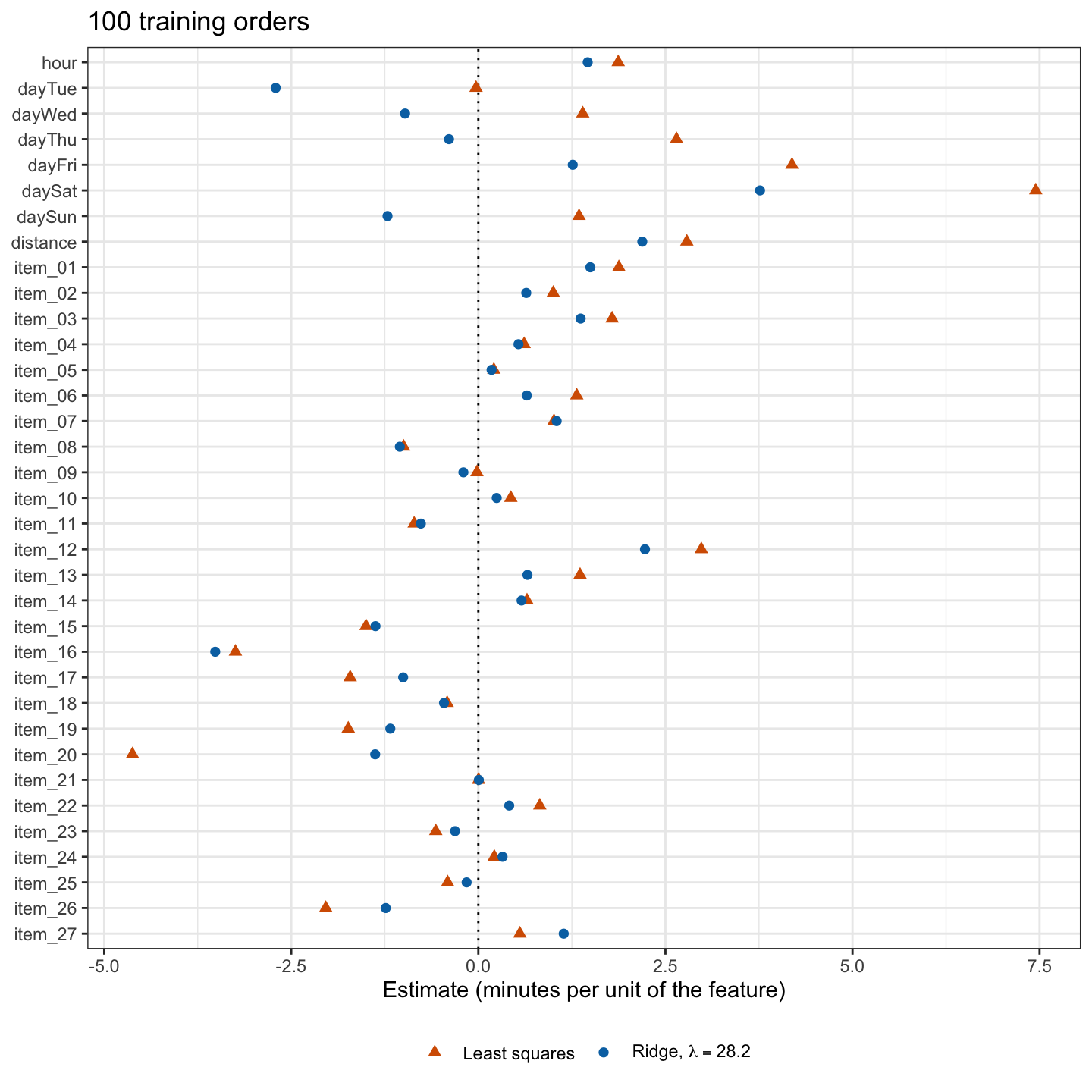
Read in order,

Intercept. On the original scale, \(\hat\beta_0 = -4.8\) minutes is the predicted time of a Monday order placed at hour 0, at distance 0, with no items, far outside the data. (The standardized-scale intercept is \(\bar y = 26.7\) minutes, the prediction at the feature means.) It sets the level: a Monday order with no items at the training orders’ mean hour, 16.2, and mean distance, 3.05 miles, has predicted time 25.6 minutes.
Hour and distance. Each hour later in the day adds 1.46 minutes (least squares: 1.87), and each mile adds 2.19 minutes (least squares: 2.79), holding the other features fixed.
Day. Each day estimate is the predicted difference from an otherwise identical order on Monday, the reference. Ridge regression lowers all 6 of them, by 2.4 to 3.7 minutes, which mostly moves Monday rather than the other days relative to each other: Saturday minus Tuesday is 7.5 minutes under least squares and 6.5 under ridge. Lowering all the day estimates by the same amount, and raising the intercept by it, changes only the predictions of Monday orders, so it shortens the vector of estimates at the cost of fitting just 4 training orders less well. Wed, Thu, and Sun, slower than Monday under least squares, are faster under ridge regression, the sign changes of the estimate path; comparisons with Monday are poorly determined by either method.
Items. Each additional unit of an item changes the predicted time by its estimate. The items that slow deliveries most are item_12, item_01, and item_03, at 2.23, 1.50, and 1.37 minutes per item. The item estimate that changes most is that of item_20, in 1 training order: -4.62 minutes per item under least squares and -1.38 under ridge regression.

The estimates are shrunken as a whole: the vector of standardized estimates has length 4.86, against 6.90 for least squares. No estimate is zero; ridge regression keeps all 35 features. Because the ridge estimator is biased toward zero, the standard errors, \(t\)-statistics, and \(p\)-values that lm() reports, which assume the unbiased least squares estimator, do not apply, and glmnet() reports none.

Beyond this course

Bayesian interpretation. If \(y_i \mid \beta \stackrel{ind}{\sim} N\left(\beta_0 + \tilde x_i\beta, \sigma^2\right)\), with \(\tilde x_i\) row \(i\) of \(\tilde{\mathbf{X}}\), and the slopes have independent priors \(\beta_j \stackrel{ind}{\sim} N\left(0, \tau^2\right)\) (with a flat prior on \(\beta_0\)), the posterior mean of \(\beta\) is the ridge estimate with \(\lambda = \sigma^2/\tau^2\).
Effective degrees of freedom. The ridge fitted values are \(\bar y\mathbf{1} + \mathbf{H}_\lambda\left(y - \bar y\mathbf{1}\right)\) with \(\mathbf{H}_\lambda = \tilde{\mathbf{X}}\mathbf{W}_\lambda\tilde{\mathbf{X}}^\top\), and \(\text{tr}\left(\mathbf{H}_\lambda\right)\) falls from \(p\) at \(\lambda = 0\) toward 0, a model size that, unlike the \(d\) of subset selection, need not be an integer.
Reference level. The penalty pulls each day estimate toward zero, that is, each day toward the reference day, so unlike least squares the ridge fit depends on which day is the reference.

21.6 Conclusion

Ridge regression keeps every feature and estimates the coefficients by minimizing \(RSS + \lambda\sum_{j=1}^p\beta_j^2\), with \(\beta_j\) the coefficients of the standardized features. Where subset selection chooses among the \(2^p\) subsets of the features, setting the estimates of the features left out exactly to zero, ridge regression shrinks all the estimates continuously. The tuning parameter \(\lambda\) sets the price of a coefficient’s size. The intercept is not penalized, so the limit as \(\lambda \to \infty\) is the null model, which predicts \(\bar y\), and the limit as \(\lambda \to 0\) is least squares. For standardized features and a centered response the estimate has the closed form \(\left(\tilde{\mathbf{X}}^\top\tilde{\mathbf{X}} + \lambda\mathbf{I}_p\right)^{-1}\tilde{\mathbf{X}}^\top\left(y - \bar y\mathbf{1}\right)\), which exists even when \(p \ge n\). Software may scale the criterion differently: glmnet()’s \(\lambda\) converts to this one by \(\lambda = n\lambda_{\text{glmnet}}/s_y\).

The penalty is not scale equivariant, so the features are standardized before fitting, and because standardization uses the data it is repeated inside every cross-validation fold. As \(\lambda\) grows the length of the vector of estimates shrinks smoothly toward zero, though correlated estimates can change sign on the way, and no estimate reaches zero. The ridge estimator is biased toward zero, but for every \(\lambda > 0\) its variance is smaller than that of the least squares estimator. Over repeated training samples, the squared bias of the predictions rises with \(\lambda\) and their variance falls, and the test MSE is smallest in between. The gain over least squares is largest when least squares has large variance, with few training observations per feature, and can vanish when it does not; and because \(\lambda\) is chosen from noisy cross-validation estimates, ridge regression can lose to least squares on a particular training sample even where it wins on average.

\(\lambda\) is chosen like any tuning parameter: by \(k\)-fold cross-validation on the training data, followed by a refit to all the training data, and the chosen model is evaluated once on test data. Ridge estimates are read like least squares estimates, but they are shrunken, and lm()’s standard errors and \(p\)-values do not apply to them.

The next lecture, the lasso, replaces the squared penalty with \(\lambda\sum_{j=1}^p\left|\beta_j\right|\), which sets some estimates exactly to zero, and compares the two on the same training and test orders.

The \(\lambda\) axis is this chapter’s \(\lambda\) only approximately. cv.glmnet() converts with the \(n\) and \(s_y\) of all 100 training orders, but each fold is fit to 90 orders with their own \(s_y\), so the \(\lambda\) a fold applies is 0.87 to 0.95 times the plotted value. Applying this chapter’s \(\lambda\) exactly in every fold gives a smallest estimate of 24.49 at \(\lambda = 25.1\); no conclusion below changes.↩︎