bike <- Bikeshare |>
  mutate(working  = factor(workingday, levels = c(0, 1),
                           labels = c("No", "Yes")),
         weather  = fct_collapse(weathersit,
                                 `rain/snow` = c("light rain/snow",
                                                 "heavy rain/snow")),
         temp_c   = 47 * temp - 8,
         hour     = as.numeric(as.character(hr)),
         hour_jit = hour + runif(n(), -0.3, 0.3))

hour_groups <- bike |>
  group_by(working, hour) |>
  summarize(n = n(), mean = mean(bikers), variance = var(bikers),
            .groups = "drop")

mv_slope <- unname(coef(lm(log(variance) ~ log(mean), data = hour_groups))[2])
busiest  <- slice_max(hour_groups, mean, n = 1)
n_heavy  <- sum(Bikeshare$weathersit == "heavy rain/snow")

# Poisson probability mass functions for the slider below.
poisson_pmf <- expand_grid(mu = seq(1, 40, by = 0.5), y = 0:70) |>
  mutate(prob = dpois(y, mu)) |>
  filter(prob > 5e-4)

count_hist_plot <- ggplot(bike, aes(x = bikers)) +
  geom_histogram(binwidth = 10, boundary = 0, fill = "grey70",
                 color = "grey40") +
  labs(x = "Bikes rented in the hour", y = "Hours",
       title = "ISLR2::Bikeshare, hourly counts")

count_hour_plot <- ggplot(bike, aes(x = hour_jit, y = bikers)) +
  geom_point(alpha = 0.08, size = 0.5) +
  geom_line(data = hour_groups, aes(x = hour, y = mean), linewidth = 0.9) +
  geom_point(data = hour_groups, aes(x = hour, y = mean), size = 1.8) +
  facet_wrap(~ working, labeller = labeller(working = working_labels)) +
  scale_x_continuous(breaks = seq(0, 24, by = 4)) +
  labs(x = "Hour of the day", y = "Bikes rented in the hour",
       title = "Hourly counts (jittered) and hourly means")

mean_variance_plot <- ggplot(hour_groups,
                             aes(x = mean, y = variance, color = working,
                                 shape = working)) +
  geom_abline(intercept = 0, slope = 1, linetype = "dashed",
              color = "grey40") +
  geom_point(size = 2.3) +
  annotate("text", x = 100, y = 55, label = "variance = mean", angle = 24,
           color = "grey30") +
  scale_x_log10(breaks = c(5, 10, 30, 100, 300)) +
  scale_y_log10() +
  scale_color_manual(values = working_colors, labels = working_labels) +
  scale_shape_manual(values = c(16, 17), labels = working_labels) +
  labs(x = "Mean count in the group (log scale)",
       y = "Variance of the count in the group (log scale)",
       color = NULL, shape = NULL,
title = "One point per hour-by-working-day group")16 Generalized Linear Models
TipLearning objectives
After this lecture you should be able to
- write a generalized linear model as its three components — a distribution for \(Y_i\) given \(x_i\) with mean \(\mu_i\), a linear predictor \(\eta_i = x_i\beta\), and a link function \(g\) with \(g(\mu_i) = \eta_i\) — and identify linear, logistic, and Poisson regression as special cases by their distribution, link, and variance,
- explain, using fitted values and residuals, why linear regression is a poor model for a count response, and contrast a linear regression of \(\log Y_i\), which models \(E[\log Y_i \mid x_i]\), with a Poisson regression, which models \(\log E[Y_i \mid x_i]\),
- write the Poisson regression log-likelihood, derive its score equations, and explain why, in general, its maximizer has no closed form,
- interpret \(e^{\beta_0}\) as a mean count and \(e^{\beta_j}\) as a rate ratio, the factor multiplying the mean count per one-unit increase in feature \(j\) with the other features held fixed, and construct Wald tests and confidence intervals for \(\beta_j\) and \(e^{\beta_j}\),
- conduct a drop-in-deviance test of a group of coefficients in a Poisson regression, and
- assess the Poisson assumption \(Var[Y_i \mid x_i] = \mu_i\) with Pearson residuals, and explain what overdispersion does to Wald standard errors and tests.
16.1 Count response
The regression lectures modeled a quantitative response whose mean could be any real number, and the logistic regression lectures a binary response whose mean is a probability. A count — the number of events in a fixed period or region — is neither: it is a nonnegative integer, its mean must be positive, and its spread typically grows with its mean.
16.1.1 Bike rentals
Question. How does the number of bikes rented in an hour depend on the time of day, whether the day is a working day, the month, the temperature, and the weather?
Data. ISLR2::Bikeshare records 8,645 hours of the Capital Bikeshare system in Washington, D.C., spread over the 365 days of one year (115 hours of the year have no record). The response is bikers, the number of bikes rented in the hour. The explanatory variables used here are
hr, the hour of the day, a factor with levels0through23,workingday, \(1\) for a day that is neither a weekend nor a holiday and \(0\) otherwise,mnth, the month, a factor,temp, the temperature rescaled to \([0, 1]\) from the range \(-8\) to \(39\) degrees Celsius, andweathersit, the weather, a factor with levelsclear,cloudy/misty,light rain/snow,heavy rain/snow.
bikers is the sum of casual and registered; those are pieces of the response, not explanatory variables, and no model below uses them.
16.1.2 Hourly counts
NoteCode
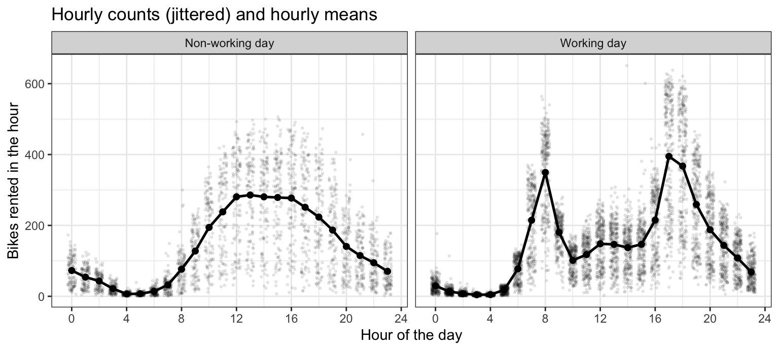
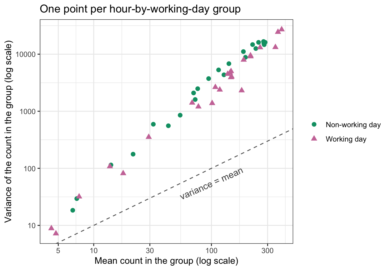
The first tab is a histogram of the hourly counts. The second plots each hour’s count, jittered horizontally, against the hour of the day, with the hourly means joined by a line, separately for non-working and working days. The third places each of the 48 hour-by-working-day groups at its mean and variance on log scales, with color and shape marking working and non-working days and a dashed line where the variance equals the mean.
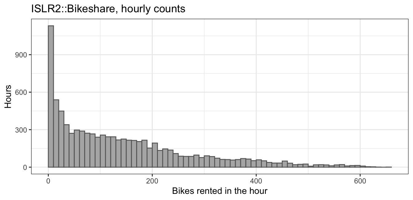
The counts run from 1 to 651 with median 109 and mean 143.8: every value is a positive integer, and the distribution is strongly right-skewed.
On working days the hourly means peak twice, at hour 8 and hour 17, the commute. On non-working days they rise to a single midday plateau. The two hourly profiles differ in shape, not just in level. Across hours, the points spread out more where the mean is higher.
In the third tab the variance climbs steadily with the mean; on these log-log axes the points lie near a line of slope 1.75. All 48 points lie above the dashed line. Month, temperature, and weather vary within each group, so part of each group’s variance is variation those explanatory variables could explain.
16.1.3 Poisson distribution
The dashed line is the variance of the standard model for a count. A count \(Y\) with a Poisson distribution with mean \(\mu\) has probability mass function
\[P(Y = y) = \frac{\mu^{y} e^{-\mu}}{y!}, \qquad y = 0, 1, 2, \ldots,\]
where
- \(\mu > 0\) is the mean, and
- \(y! = 1 \times 2 \times \cdots \times y\), with \(0! = 1\).
ISLR2 writes \(\lambda\) for the Poisson mean; these notes write \(\mu\), the symbol the generalized linear models below use for a mean.
The mean and the variance are both \(\mu\). Dropping the \(y = 0\) term and cancelling \(y\) against \(y!\),
\[E[Y] = \sum_{y=1}^\infty y\, \frac{\mu^{y} e^{-\mu}}{y!} = \mu \sum_{y=1}^\infty \frac{\mu^{y-1} e^{-\mu}}{(y-1)!} = \mu,\]
because the last sum adds the probability mass function over every count. The same step applied twice gives \(E[Y(Y - 1)] = \mu^2\), so
\[Var[Y] = E[Y(Y - 1)] + E[Y] - \mu^2 = \mu^2 + \mu - \mu^2 = \mu.\]
The slider below moves \(\mu\). The black lollipops are the probability mass function, the dashed line marks the mean, the shaded band runs one standard deviation, \(\sqrt{\mu}\), either side of it; both axes rescale as \(\mu\) moves, so read the spread and the heights from the axis labels.
At a mean near \(1\) most of the probability sits at \(0\), \(1\), and \(2\), and the distribution is strongly right-skewed. As \(\mu\) grows the distribution moves right, becomes nearly symmetric, and widens: its standard deviation \(\sqrt\mu\) grows with its mean. The slider stops at \(40\). The busiest bike group, with mean 395, would have Poisson standard deviation 19.9; its observed standard deviation is 164.4 (variance 27,031), the gap the mean–variance plot showed for every group.
16.1.4 Linear regression fails
A linear regression fit by least squares uses these features:
- 23 dummy features for
hr, with hour0the reference, - the indicator \(\mathrm{I}(\texttt{workingday} = 1)\),
- 23 products of each hour dummy with the working-day indicator, because the two hourly profiles differ in shape,
- 11 dummy features for
mnth, with January the reference, - the temperature in degrees Celsius, the feature \(h(\texttt{temp}) = 47\,\texttt{temp} - 8\), and
- 2 dummy features for the weather, with
clearthe reference, after mergingheavy rain/snowintolight rain/snowasrain/snow, sinceheavy rain/snowoccurs in 1 hour.
bike_formula <- bikers ~ hr * working + mnth + temp_c + weather
bike_lm <- lm(bike_formula, data = bike)
NoteCode
bike <- bike |>
  mutate(fit_lm = fitted(bike_lm), resid_lm = residuals(bike_lm))

n_negative <- sum(bike$fit_lm < 0)
fit_low  <- 50
fit_high <- 300
sd_low  <- sd(bike$resid_lm[bike$fit_lm < fit_low])
sd_high <- sd(bike$resid_lm[bike$fit_lm > fit_high])
b_lm    <- coef(bike_lm)

lm_residual_plot <- ggplot(bike, aes(x = fit_lm, y = resid_lm)) +
  geom_point(alpha = 0.1, size = 0.6) +
  geom_vline(xintercept = 0, linetype = "dashed", color = "#D55E00") +
  geom_hline(yintercept = 0, color = "grey40") +
  labs(x = "Fitted value from least squares",
       y = "Residual", title = "Linear regression residuals")
The figure plots each hour’s residual against its least squares fitted value; the dashed vertical line marks a fitted value of zero and the solid horizontal line a residual of zero.
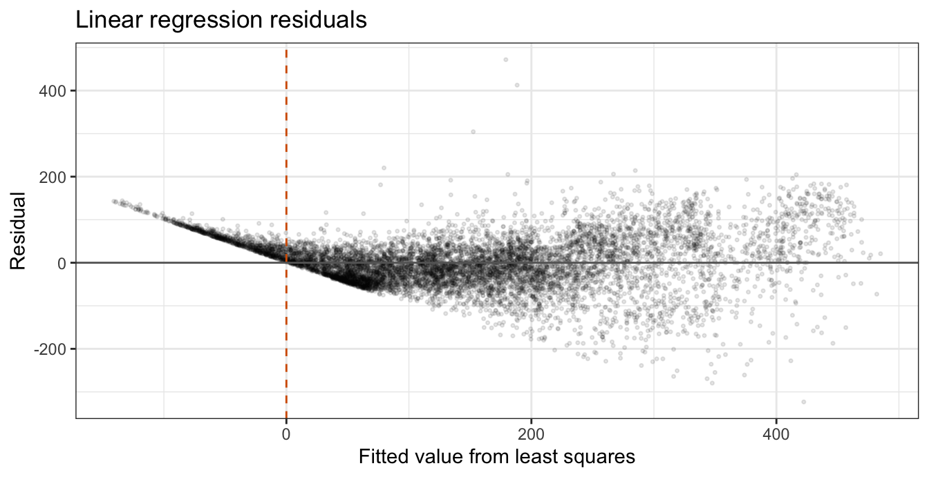
Three failures appear.
- Negative fitted means. Every point left of the dashed line has a negative fitted value: 895 of the 8,645 hours, 10.4%, with the smallest at -140.9 bikers. A mean count cannot be negative.
- Variance growing with the mean. The residuals fan out to the right. Their standard deviation is 37.6 among hours with fitted values below \(50\) and 90.5 among hours with fitted values above \(300\), while every \(t\)-test and interval from
lm()assumes one common variance. - Additive effects. Every additive effect — month, temperature, and weather — shifts every hour by the same number of riders. Within each combination of hour and working-day status, an hour whose shift is smaller than average — a winter month, a cold hour, rain — sits the same number of riders below the combination’s mean at 3 a.m. as at 5 p.m., and at night that is enough to push the fit below zero: 460 of the 895 negative fitted values are in clear weather, and the median temperature of all 895 is 3.3 degrees Celsius, against 15.5 for all hours.
16.1.5 Log-count linear regression
The regression lectures’ remedy for a positive response whose spread grows with its mean is least squares on \(\log Y_i\) with the same features. Its model is
\[\log Y_i \mid x_i \stackrel{ind}{\sim} N\left(x_i\gamma, \sigma^2\right),\]
where
- \(x_i = (1, x_{i1}, \ldots, x_{ip})\) is the \(i\)th row of the model matrix \(\mathbf{X}\): a leading \(1\) and the 61 features of the linear regression above, and
- \(\gamma = (\gamma_0, \ldots, \gamma_p)^\top\) and \(\sigma^2\) are this model’s coefficients and error variance, estimated by least squares and the residual mean square.
A fitted value \(x_i\hat\gamma\) is on the log scale. Exponentiated,
\[e^{x_i\hat\gamma} = e^{\hat\gamma_0} \times e^{\hat\gamma_1 x_{i1}} \times \cdots \times e^{\hat\gamma_p x_{ip}}\]
is positive for every \(\hat\gamma\), and each feature multiplies it by a factor rather than adding a number of riders, which addresses the first and third failures. Counting the hours with zero bikers, then fitting with the features of bike_formula:
sum(bike$bikers == 0)[1] 0bike_log_lm <- lm(update(bike_formula, log(.) ~ .), data = bike)No hour has zero bikers (the count is 0), so \(\log y_i\) is defined for all 8,645 hours.
NoteCode
bike <- bike |>
  mutate(fit_log   = exp(fitted(bike_log_lm)),
         resid_log = residuals(bike_log_lm))

sd_low_log  <- sd(bike$resid_log[bike$fit_log < fit_low])
sd_high_log <- sd(bike$resid_log[bike$fit_log > fit_high])

combination_log <- bike |>
  group_by(working, hour) |>
  summarize(ratio = mean(fit_log) / mean(bikers), .groups = "drop")

log_residual_plot <- ggplot(bike, aes(x = fitted(bike_log_lm),
                                      y = resid_log)) +
  geom_point(alpha = 0.1, size = 0.6) +
  geom_hline(yintercept = 0, color = "grey40") +
  labs(x = "Fitted log count from least squares",
       y = "Residual (log scale)",
       title = "Log-count linear regression residuals")
The figure plots each hour’s residual against its fitted log count; the solid line marks a residual of zero.
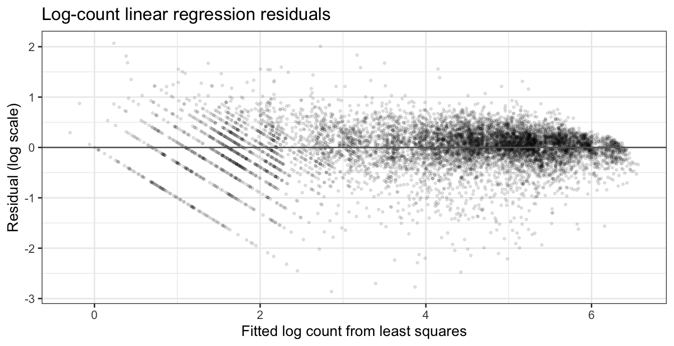
The smallest back-transformed fitted value is 0.75 bikers, so no fitted value is negative. The residuals no longer fan out to the right; they narrow instead. Their standard deviation is 0.55 among hours with back-transformed fitted values below \(50\) and 0.23 among hours with back-transformed fitted values above \(300\): on the log scale the spread shrinks as the mean grows, so the one common variance \(\sigma^2\) still does not describe the data.
The model also changes what is estimated. Exponentiating a fitted value gives \(e^{x_i\hat\gamma}\), a positive number on the scale of the counts, but it estimates \(e^{E[\log Y_i \mid x_i]}\), not the mean count. Jensen’s inequality states that \(E[g(Y)] \le g(E[Y])\) for a concave function \(g\); with \(g = \log\) it gives \(E[\log Y_i \mid x_i] \le \log E[Y_i \mid x_i]\), and therefore
\[e^{E[\log Y_i \mid x_i]} \le E[Y_i \mid x_i],\]
with equality only when \(Y_i\) given \(x_i\) is constant. Under the normal model \(\log Y_i\) has median \(x_i\gamma\), and the exponential is increasing, so \(e^{x_i\gamma}\) is the median of \(Y_i\) given \(x_i\): the median reading of a logged response in the Multiple (Linear) Regression lecture.
Averaged within each of the 48 combinations of hour and working-day status, the back-transformed fitted values fall below the observed mean in 45, with a median ratio to the observed mean of 0.93.
16.2 Generalized linear models
The figure repeats the mean–variance plot of the hourly counts: each of the 48 hour-by-working-day groups at its mean and variance on log scales, with color and shape marking working and non-working days and a dashed line where the variance equals the mean.
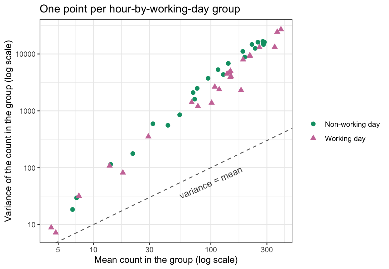
The variance grows with the mean, and much faster than the constant variance the linear regression assumed. A generalized linear model lets the distribution, and with it the way the variance depends on the mean, change with the response. The Problems in Logistic Regression lecture wrote each model as one distributional statement: \(Y_i \mid x_i \stackrel{ind}{\sim} N(x_i\beta, \sigma^2)\) for linear regression, and \(Y_i \mid x_i \stackrel{ind}{\sim} \text{Bernoulli}\left[p(x_i)\right]\) with \(\log\left[\frac{p(x_i)}{1 - p(x_i)}\right] = x_i\beta\) for logistic regression. Both statements have the same three parts — a distribution, a linear predictor, and a link — and generalized linear models keep those parts while letting each one vary.
16.2.1 Three components
A generalized linear model (GLM) assumes the statistical model
\[Y_i \mid x_i \stackrel{ind}{\sim} \text{a distribution with mean } \mu_i, \qquad g(\mu_i) = \eta_i, \qquad \eta_i = x_i\beta,\]
where
- \(\mu_i = E[Y_i \mid x_i]\) is the mean of the response of observation \(i\) (unrelated to the class means \(\mu_k\) of the discriminant analysis lectures),
- \(x_i = (1, x_{i1}, \ldots, x_{ip})\) is the \(i\)th row of the model matrix \(\mathbf{X}\) and \(\beta = (\beta_0, \ldots, \beta_p)^\top\) is the vector of coefficients,
- \(\eta_i\) is the linear predictor, as in the problems lecture, and
- \(g\) is the link function, a strictly monotone function (ISLR2 writes \(\eta\) for the link itself; these notes write \(g\)).
The distribution of \(Y_i\) given \(x_i\) is the random component. The linear predictor is where the features enter: dummy variables, polynomials, step functions, and interactions enter it exactly as they entered a linear or logistic regression. The link connects the two; inverting it, \(\mu_i = g^{-1}(\eta_i) = g^{-1}(x_i\beta)\).
The link is what keeps the mean in range. A linear predictor can take any real value, and for the identity, logit, and log links used in this lecture \(g^{-1}\) carries the real line onto the values the mean is allowed to take — \((0, 1)\) for a probability, \((0, \infty)\) for a count — so every \(\beta\) gives a valid mean.
For the bike counts, \(Y_i\) is bikers in hour \(i\), and \(x_i\) is the row of 62 entries — a leading \(1\) and the features of the linear regression above — so \(\eta_i\) is the same linear predictor in the linear regression above and in the Poisson regression introduced below. The linear regression is the GLM with a normal random component and the identity link, \(g(\mu_i) = \mu_i\), which does nothing to keep \(x_i\hat\beta\) positive: that is how 895 of its fitted means fell below zero.
16.2.2 Special cases
NoteCode
glm_table <- tibble(
  Model = c("Linear regression", "Logistic regression", "Poisson regression"),
  Response = c("Quantitative", "Binary ($0/1$)", "Count"),
  Distribution = c("$N(\\mu_i, \\sigma^2)$", "$\\text{Bernoulli}(\\mu_i)$",
                   "$\\text{Poisson}(\\mu_i)$"),
  Link = c("identity, $\\mu_i$", "logit, $\\log\\left[\\mu_i/(1 - \\mu_i)\\right]$",
           "log, $\\log \\mu_i$"),
  Mean = c("$\\eta_i$", "$e^{\\eta_i}/\\left(1 + e^{\\eta_i}\\right)$",
           "$e^{\\eta_i}$"),
  Variance = c("$\\sigma^2$", "$\\mu_i(1 - \\mu_i)$", "$\\mu_i$"),
  family = c("`gaussian`", "`binomial`", "`poisson`")
) |>
  knitr::kable(col.names = c("Model", "Response", "Distribution of $Y_i$",
                             "Link $g(\\mu_i)$", "Mean $\\mu_i$",
                             "Variance", "`glm()` family"),
               align = "lllllll")
For each model the table gives the response type, the distribution of \(Y_i\), the link, the mean as a function of \(\eta_i\), the variance, and the glm() family that fits it (family = gaussian gives the same estimates as lm()).
| Model | Response | Distribution of \(Y_i\) | Link \(g(\mu_i)\) | Mean \(\mu_i\) | Variance | glm() family |
|---|---|---|---|---|---|---|
| Linear regression | Quantitative | \(N(\mu_i, \sigma^2)\) | identity, \(\mu_i\) | \(\eta_i\) | \(\sigma^2\) | gaussian |
| Logistic regression | Binary (\(0/1\)) | \(\text{Bernoulli}(\mu_i)\) | logit, \(\log\left[\mu_i/(1 - \mu_i)\right]\) | \(e^{\eta_i}/\left(1 + e^{\eta_i}\right)\) | \(\mu_i(1 - \mu_i)\) | binomial |
| Poisson regression | Count | \(\text{Poisson}(\mu_i)\) | log, \(\log \mu_i\) | \(e^{\eta_i}\) | \(\mu_i\) | poisson |
In logistic regression the mean \(\mu_i = P(Y_i = 1 \mid x_i)\) is the probability the Simple Logistic Regression lecture and its successors wrote \(p(x_i)\); those lectures, with the credit card default data, are this table’s logistic regression row.
Each distribution fixes how the variance depends on the mean,
\[Var[Y_i \mid x_i] = \phi\, V(\mu_i),\]
where
- \(V\) is the variance function: \(V(\mu) = 1\) for the normal, \(V(\mu) = \mu(1 - \mu)\) for the Bernoulli, and \(V(\mu) = \mu\) for the Poisson, and
- \(\phi\) is the dispersion parameter: \(\phi = \sigma^2\) for the normal, and \(\phi = 1\) for the Bernoulli and the Poisson, which have no variance parameter separate from the mean.
Linear regression’s constant variance is the special case \(V(\mu) = 1\), the assumption the fanning residuals of the bike-count linear regression contradicted. The two other models require the variance to change with the mean, as the bike counts’ variance did in the mean–variance plot.
A GLM transforms the mean, not the response. Both the log-count linear regression above and the Poisson regression below put the linear predictor on a log scale, but of different quantities:
\[\text{log-count linear regression: } E[\log Y_i \mid x_i] = x_i\gamma, \qquad \text{Poisson regression: } \log E[Y_i \mid x_i] = x_i\beta.\]
The log-count model takes the logarithm of \(y_i\), so it fails for a count of zero (bikers has none, but counts in general can); a log link never takes the logarithm of \(y_i\).
NoteBeyond this course
The three distributions belong to the exponential family, and each row uses its canonical link, under which the score equations take the form \(\sum_i x_{ij}(y_i - \mu_i) = 0\) derived below. The same template covers other distributions, other links, and more than two classes:
- Gamma regression, for a positive, right-skewed response such as a claim amount, has \(V(\mu) = \mu^2\):
family = Gamma(link = "log"). - Probit regression keeps the Bernoulli and uses the inverse standard normal cumulative distribution function as link:
binomial(link = "probit"). - Multinomial logistic regression, for an unordered response with \(K > 2\) classes (ISLR2 Section 4.3.5), extends the Bernoulli to a categorical distribution with \(K - 1\) linear predictors, one for each class other than a reference class; it is fit with
nnet::multinom(). - Ordinal (proportional-odds) regression, for ordered classes, uses one linear predictor together with \(K - 1\) cutpoints; it is fit with
MASS::polr().
None of these is taught or tested here.
16.3 Poisson regression
NoteCode
cell_means <- bike |>
  group_by(weather, working, hour) |>
  summarize(n = n(), observed = mean(bikers), .groups = "drop")

observed_points <- geom_point(aes(shape = "Observed mean"), size = 1.3)

# Axes, facets, and scales without the points, so later figures can draw
# fitted lines underneath the points.
observed_frame <- ggplot(cell_means, aes(x = hour, y = observed)) +
  geom_hline(yintercept = 0, color = "grey50", linetype = "dotted") +
  facet_grid(weather ~ working, scales = "free_y",
             labeller = labeller(working = working_labels)) +
  scale_x_continuous(breaks = seq(0, 24, by = 4)) +
  scale_shape_manual(values = c("Observed mean" = 1)) +
  labs(x = "Hour of the day", y = "Mean bikes rented in the hour",
       color = NULL, linetype = NULL, shape = NULL) +
  theme(legend.position = "none")

observed_plot <- observed_frame + observed_points +
  labs(title = "Observed hourly means")

# Rain/snow vs. clear on working days: ratio and difference of hourly means.
rain_vs_clear <- cell_means |>
  filter(working == "Yes", weather %in% c("clear", "rain/snow")) |>
  pivot_wider(id_cols = hour, names_from = weather, values_from = observed) |>
  mutate(ratio = `rain/snow` / clear, diff = clear - `rain/snow`)
at_3  <- unlist(filter(rain_vs_clear, hour == 3))
at_17 <- unlist(filter(rain_vs_clear, hour == 17))
The figure splits the hours by weather (rows) and working-day status (columns); each point is the observed mean count for one hour of the day in that panel, each row has its own vertical scale, and the dotted line marks zero.
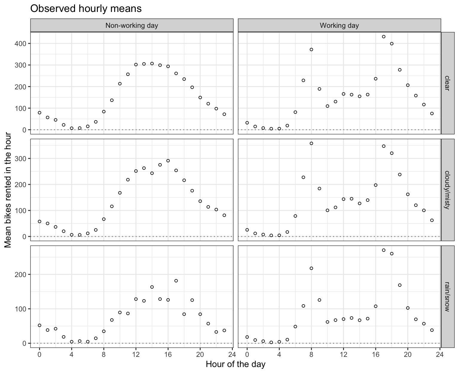
Each weather row repeats the hourly profile of the clear row at a lower level. On working days the rain/snow mean is 0.54 times the clear mean at 3 a.m. and 0.63 times at 5 p.m., while the differences are 2.2 and 161.1 riders: rain scales the profile, which is a multiplicative effect, rather than lowering every hour by the same number.
16.3.1 Log-linear model
Poisson regression is the GLM with a Poisson random component and a log link:
\[Y_i \mid x_i \stackrel{ind}{\sim} \text{Poisson}(\mu_i), \qquad \log \mu_i = x_i\beta = \beta_0 + \beta_1 x_{i1} + \cdots + \beta_p x_{ip}.\]
Inverting the link,
\[\mu_i = e^{x_i\beta} = e^{\beta_0} \times e^{\beta_1 x_{i1}} \times \cdots \times e^{\beta_p x_{ip}},\]
which is positive for every \(\beta\) and every row \(x_i\). The features add on the log scale and multiply on the scale of the mean. A weather dummy therefore multiplies every hour’s mean by the same factor \(e^{\beta_j}\), the scaling of the rain/snow row in the figure above.
16.3.2 Maximum likelihood estimation
For independent observations the log-likelihood is the sum of the logarithms of the probability mass functions,
\[\ell(\beta) = \sum_{i=1}^n \left[y_i \log \mu_i - \mu_i - \log(y_i!)\right] = \sum_{i=1}^n \left[y_i\, x_i\beta - e^{x_i\beta} - \log(y_i!)\right],\]
where
- \(y_i\) is the observed count for observation \(i\), and
- \(\log(y_i!)\) does not involve \(\beta\) and so does not affect the maximizer.
Differentiating with respect to \(\beta_j\), using \(\partial e^{x_i\beta} / \partial \beta_j = x_{ij} e^{x_i\beta}\), and setting the result to zero gives the score equations
\[\sum_{i=1}^n x_{ij}\left(y_i - \mu_i\right) = 0, \qquad j = 0, 1, \ldots, p,\]
with \(x_{i0} = 1\). They have exactly the form of the logistic regression score equations with \(\mu_i\) in place of \(p(x_i)\): at the solution the residuals \(y_i - \hat\mu_i\), where \(\hat\mu_i = e^{x_i\hat\beta}\) is the fitted mean, sum to zero and are orthogonal to every feature. Because \(\mu_i = e^{x_i\beta}\) is nonlinear in \(\beta\), the equations in general have no closed-form solution: with only the hour-by-working-day dummies the solution is the cell means (which the score check below shows the fit reproduces), but with a quantitative feature such as temperature it has none.
glm() solves them with the iterative algorithm it used for logistic regression, iteratively reweighted least squares: each iteration solves a weighted least squares problem whose weights are recomputed from the current estimate. Fitting the bike counts with the features of the linear regression:
bike_glm <- glm(bike_formula, data = bike, family = poisson)summary() reports each coefficient’s estimate, standard error, Wald \(z\) statistic, and \(p\)-value. Of the 62 coefficients, these are the intercept and the coefficients for working day, temperature, and weather:
printCoefmat(summary(bike_glm)$coefficients[
  c("(Intercept)", "workingYes", "temp_c", "weathercloudy/misty",
    "weatherrain/snow"), ])
Estimate Std. Error z value Pr(>|z|)
(Intercept) 3.36291632 0.01208439 278.286 < 2.2e-16 ***
workingYes -0.91915334 0.01608340 -57.149 < 2.2e-16 ***
temp_c 0.01605829 0.00024332 65.998 < 2.2e-16 ***
weathercloudy/misty -0.06709450 0.00218683 -30.681 < 2.2e-16 ***
weatherrain/snow -0.58063152 0.00406292 -142.910 < 2.2e-16 ***
---
Signif. codes: 0 '***' 0.001 '**' 0.01 '*' 0.05 '.' 0.1 ' ' 1
NoteCode
bike <- bike |>
  mutate(fit_glm = fitted(bike_glm))

combination_gap <- bike |>
  group_by(working, hour) |>
  summarize(gap_glm = abs(mean(bikers) - mean(fit_glm)),
            gap_lm  = abs(mean(bikers) - mean(fit_lm)), .groups = "drop")
max_gap <- max(combination_gap$gap_glm, combination_gap$gap_lm)
The model has 62 coefficients, as the linear regression does, and glm() reports convergence after 4 iterations. The intercept’s score equation makes the fitted means sum to the observed counts, \(\sum_i \hat\mu_i = 1{,}243{,}103\) and \(\sum_i y_i = 1{,}243{,}103\). A dummy variable’s equation makes the fitted means average to the observed mean where that dummy is \(1\), as the least squares normal equations also do, so both models reproduce the observed mean of each of the 48 combinations of hour and working-day status (largest gap \(6.9 \times 10^{-8}\) bikers).
16.3.3 Fitted means
NoteCode
cell_fits <- bike |>
  group_by(weather, working, hour) |>
  summarize(`Linear regression` = mean(fit_lm),
            `Log-count linear regression` = mean(fit_log),
            `Poisson regression` = mean(fit_glm), .groups = "drop") |>
  right_join(cell_means, by = c("weather", "working", "hour"))

cell_long <- cell_fits |>
  pivot_longer(all_of(names(model_colors)),
               names_to = "model", values_to = "fitted") |>
  mutate(model = factor(model, levels = names(model_colors)))

rain_night <- filter(cell_fits, weather == "rain/snow", hour <= 6)
n_below <- sapply(names(model_colors),
                  function(m) sum(cell_fits[[m]] < cell_fits$observed))

fitted_plot <- observed_frame +
  geom_line(data = cell_long,
            aes(y = fitted, color = model, linetype = model),
            linewidth = 0.8) +
  observed_points +
  scale_color_manual(values = model_colors) +
  scale_linetype_manual(values = model_linetypes) +
  guides(shape = guide_legend(order = 1),
         color = guide_legend(order = 2),
         linetype = guide_legend(order = 2)) +
  labs(title = "Observed and fitted hourly means") +
  theme(legend.position = "bottom",
        legend.key.width = unit(2.5, "lines"))
The figure redraws the observed hourly means of the figure above and adds one line per model through its fitted means, averaged within each point’s group; for the log-count linear regression the fitted values are the back-transformed \(e^{x_i\hat\gamma}\).
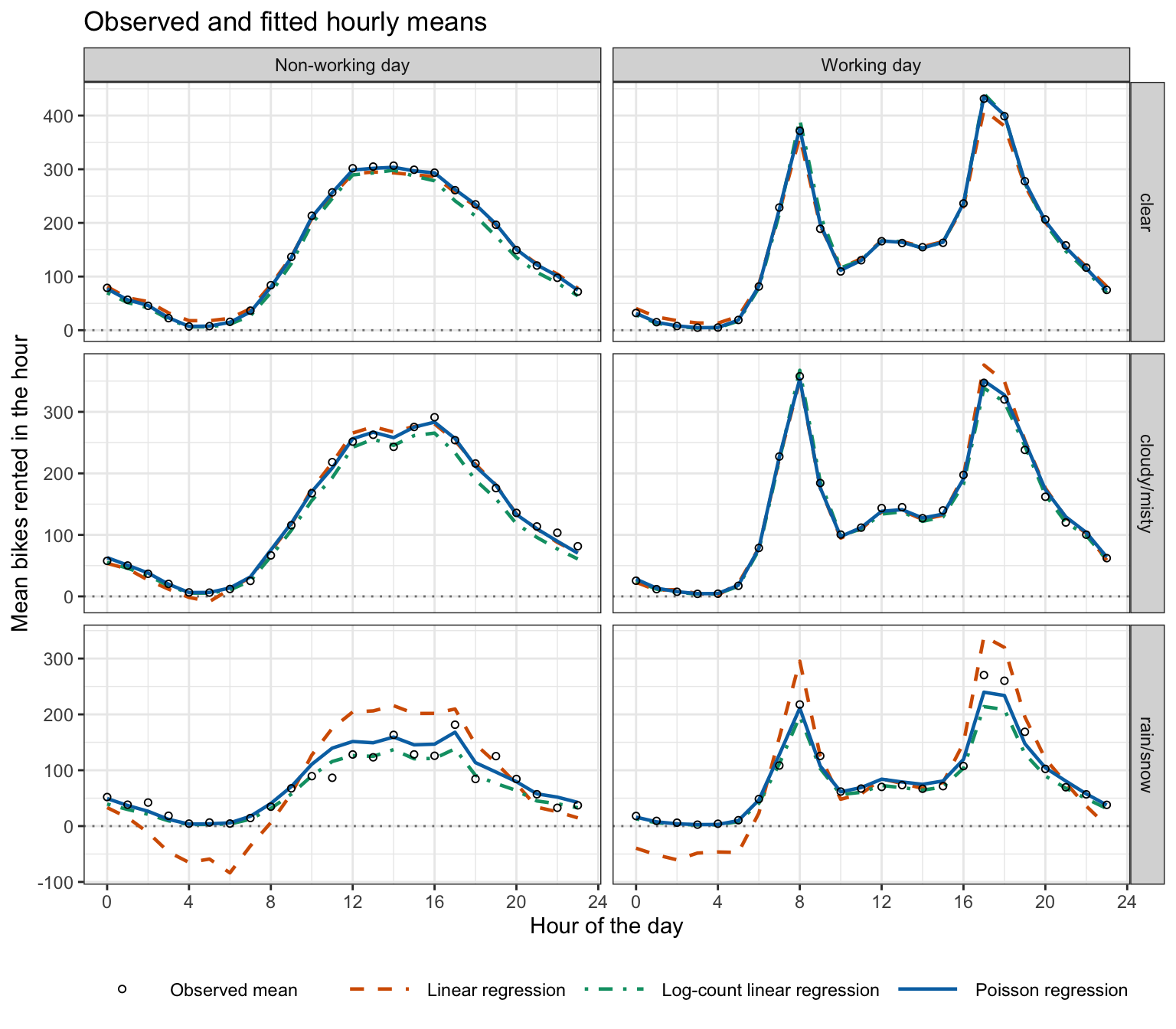
Pooled over weather, linear and Poisson regression agree, since both reproduce each hour-by-working-day mean; they differ only in how they split each combination across the weather rows. In the rain/snow row, linear regression subtracts its constant weather coefficient from every hour, and its lines fall below zero overnight and in the early morning, as low as -83.7 bikers, where the observed means never fall below 2.6. The Poisson lines scale the hourly profile down instead and follow the points much more closely, overnight included.
The log-count lines also scale the profile and stay positive; their smallest overnight value in the rain/snow row is 2.1 bikers. Across all panels they lie below the observed mean at 122 of the 144 points, against 68 for the Poisson lines. Summed over all hours, the back-transformed fitted values total 1,202,378 bikers, against the 1,243,103 observed, a total the Poisson fitted means reproduce. Both comparisons are consistent with a fit that estimates \(e^{E[\log Y_i \mid x_i]}\) rather than the mean count.
16.3.4 Coefficient interpretation
Write \(\mu(x)\) for the mean count at a row of feature values \(x = (1, x_1, \ldots, x_p)\). At \(x = (1, 0, \ldots, 0)\), \(\log \mu(x) = \beta_0\), so \(e^{\beta_0}\) is the mean count when every feature is zero — for dummy variables, at the reference levels.
Increasing feature \(j\) by one unit from \(x_j\) while holding every other feature fixed, every term of the linear predictor except the \(j\)th cancels:
\[\log \mu(x_j + 1) - \log \mu(x_j) = \beta_j, \qquad \frac{\mu(x_j + 1)}{\mu(x_j)} = e^{\beta_j},\]
where
- \(\mu(x_j)\) and \(\mu(x_j + 1)\) are the mean counts at two feature rows that differ only in feature \(j\), by one unit.
So \(\beta_j\) is the change in the log mean count per one-unit increase in \(x_j\), and \(e^{\beta_j}\), the rate ratio, is the factor multiplying the mean count, holding the other features fixed — the odds ratio of logistic regression with the mean count in place of the odds. \(e^{\beta_j} = 1\) means no association; \(c\) units multiply the mean by \(e^{c\beta_j}\); for a dummy variable, \(e^{\beta_j}\) is the mean at the indicated level divided by the mean at the reference level; and with an interaction \(x_j x_l\) the rate ratio for \(x_j\) depends on \(x_l\).
NoteCode
b     <- coef(bike_glm)
shown <- c("(Intercept)", "workingYes", "temp_c", "weathercloudy/misty",
           "weatherrain/snow")
shown_labels <- c("Intercept", "Working day (at hour 0)",
                  "Temperature (per degree C)", "Cloudy/misty vs. clear",
                  "Rain/snow vs. clear")

rate_ratio_table <- tibble(
  Coefficient = shown_labels,
  Estimate = sprintf("%.4f", b[shown]),
  exp_b = sprintf("%.4f", exp(b[shown]))
) |>
  knitr::kable(col.names = c("Coefficient", "Estimate",
                             "$e^{\\hat\\beta_j}$"),
               align = "lcc")

z  <- summary(bike_glm)$coefficients[, "z value"]
ci <- confint.default(bike_glm)
rr_ci <- function(term, c = 1) {
  sprintf("(%.3f, %.3f)", exp(c * ci[term, 1]), exp(c * ci[term, 2]))
}

rr_working_8 <- exp(b["workingYes"] + b["hr8:workingYes"])
rr_temp_5    <- exp(5 * b["temp_c"])
rr_rain      <- exp(b["weatherrain/snow"])
For the bike counts, the intercept and the coefficients for working day, temperature, and weather, with their exponentials:
| Coefficient | Estimate | \(e^{\hat\beta_j}\) |
|---|---|---|
| Intercept | 3.3629 | 28.8733 |
| Working day (at hour 0) | -0.9192 | 0.3989 |
| Temperature (per degree C) | 0.0161 | 1.0162 |
| Cloudy/misty vs. clear | -0.0671 | 0.9351 |
| Rain/snow vs. clear | -0.5806 | 0.5595 |
\(e^{\hat\beta_0} = 28.9\) is the estimated mean count at hour \(0\) (midnight to 1 a.m.) on a non-working day in January, in clear weather at \(0\) degrees Celsius — a realistic winter night, unlike the linear regression’s intercept of -10.9 bikers for the same conditions.
Because hour and working day interact, the working-day coefficient compares the two kinds of day at the reference hour only: at midnight a working day’s estimated mean is \(e^{\hat\beta_{\texttt{workingYes}}} = 0.40\) times a non-working day’s. At 8 a.m. the corresponding ratio adds the hr8:workingYes coefficient to the exponent, \(e^{-0.919 +2.442} = 4.59\).
Holding hour, working-day status, month, and weather fixed, each additional degree Celsius multiplies the estimated mean count by 1.0162, so \(5\) degrees multiply it by \(e^{5\hat\beta_{\texttt{temp}\_\texttt{c}}} = 1.084\), an increase of 8.4%.
Rain or snow multiplies the estimated mean by 0.560 relative to clear weather — a 44% reduction at every hour, month, and temperature, the scaling seen in the rain/snow row of the fitted-means figure — and cloudy or misty weather multiplies it by 0.935.
16.3.5 Inference
Inference repeats the logistic regression lectures. In large samples \(\hat\beta_j\) is approximately normal, so
\[z = \frac{\hat\beta_j - \beta_j^0}{\text{SE}\left(\hat\beta_j\right)}\]
is approximately standard normal under \(H_0: \beta_j = \beta_j^0\), where \(\text{SE}\left(\hat\beta_j\right)\) comes from the curvature of \(\ell\) at \(\hat\beta\). The Wald interval \(\hat\beta_j \pm z_{1-\alpha/2}\,\text{SE}\left(\hat\beta_j\right)\) is returned by confint.default(), and exponentiating its endpoints gives an interval for the rate ratio \(e^{\beta_j}\).
For the four rate ratios of the bike-count table, \(|z|\) ranges from 30.7 to 142.9, and the 95% intervals are \((0.386, 0.412)\) for working day at hour \(0\), \((1.081, 1.086)\) per \(5\) degrees Celsius, \((0.931, 0.939)\) for cloudy or misty weather, and \((0.555, 0.564)\) for rain or snow: every one excludes \(1\).
A group of coefficients — every product of an hour dummy with the working-day indicator, say — is tested with the drop-in-deviance test. For a count response glm() reports the residual deviance
\[D = 2\left[\ell_{\text{sat}} - \ell\left(\hat\beta\right)\right],\]
where
- \(D\) is the deviance, as in the Multiple Logistic Regression lecture, not an indicator variable, and
- \(\ell_{\text{sat}}\) is the log-likelihood of the saturated model, which gives each observation its own mean \(\mu_i = y_i\), the largest log-likelihood any mean model can reach.
\(\ell_{\text{sat}}\) does not involve \(\beta\), so for a reduced model nested in a full one, \(G^2 = D_r - D_f = -2\left[\ell\left(\hat\beta_r\right) - \ell\left(\hat\beta_f\right)\right]\), the drop-in-deviance statistic of the multiple logistic regression lecture. (For a binary response \(\ell_{\text{sat}} = 0\), which is why that lecture could write \(D = -2\ell\left(\hat\beta\right)\).) Under \(H_0\) that the \(k\) dropped coefficients are zero, \(G^2\) is approximately \(\chi^2_k\), and anova(reduced, full, test = "Chisq") performs the test.
The bike-count model’s 23 hour-by-working-day products are such a group: no single \(z\)-test asks whether working and non-working days share one hourly profile up to a constant factor. The test compares the full model with the additive one:
bike_additive <- glm(bikers ~ hr + working + mnth + temp_c + weather,
                     data = bike, family = poisson)
interaction_test <- anova(bike_additive, bike_glm, test = "Chisq")
interaction_test
Analysis of Deviance Table
Model 1: bikers ~ hr + working + mnth + temp_c + weather
Model 2: bikers ~ hr * working + mnth + temp_c + weather
Resid. Df Resid. Dev Df Deviance Pr(>Chi)
1 8606 228046
2 8583 99377 23 128669 < 2.2e-16 ***
---
Signif. codes: 0 '***' 0.001 '**' 0.01 '*' 0.05 '.' 0.1 ' ' 1G2 <- interaction_test$Deviance[2]
k <- interaction_test$Df[2]The deviance drops by \(G^2 = 128{,}669\) on \(k = 23\) degrees of freedom, against a \(\chi^2_{23}\) mean of 23. The data are inconsistent with one hourly profile, up to a constant factor, shared by both kinds of day.
16.3.6 Overdispersion
The Poisson model has no variance parameter: \(Var[Y_i \mid x_i] = \mu_i\), and every standard error and deviance test above is computed under that variance. Overdispersion is the failure \(Var[Y_i \mid x_i] > \mu_i\).
The Pearson residual \(\left(y_i - \hat\mu_i\right)/\sqrt{\hat\mu_i}\) standardizes a residual by the Poisson standard deviation. If \(Var[Y_i \mid x_i] = \mu_i\), then \(E\left[(Y_i - \mu_i)^2/\mu_i \mid x_i\right] = 1\), so the average squared Pearson residual,
\[\hat\phi = \frac{1}{n - (p+1)}\sum_{i=1}^n \frac{\left(y_i - \hat\mu_i\right)^2}{\hat\mu_i},\]
should be close to \(1\), and a value well above \(1\) is evidence of overdispersion, where
- \(\hat\phi\) estimates the dispersion parameter \(\phi\), which the Poisson model fixes at \(1\), and
- the divisor \(n - (p+1)\) accounts for the \(p + 1\) estimated coefficients, as in \(\hat\sigma^2 = RSS/[n - (p+1)]\).
NoteCode
pearson_phi <- function(fit) {
  sum(residuals(fit, type = "pearson")^2) / df.residual(fit)
}
phi_full     <- pearson_phi(bike_glm)
phi_additive <- pearson_phi(bike_additive)

n_bins <- 20
variance_bins <- bike |>
  mutate(bin = ntile(fit_glm, n_bins)) |>
  group_by(bin) |>
  summarize(mean_fit = mean(fit_glm),
            mean_sq_resid = mean((bikers - fit_glm)^2), .groups = "drop")

variance_check_plot <- ggplot(variance_bins,
                              aes(x = mean_fit, y = mean_sq_resid)) +
  geom_abline(intercept = 0, slope = 1, linetype = "dashed",
              color = "grey40") +
  geom_point(size = 2.3) +
  annotate("text", x = 100, y = 55, label = "Poisson: variance = mean",
           angle = 24, color = "grey30") +
  scale_x_log10() +
  scale_y_log10() +
  labs(x = expression(paste("Average ", hat(mu)[i], " in the bin (log scale)")),
       y = expression(paste("Average ", (y[i] - hat(mu)[i])^2,
                            " in the bin (log scale)")),
       title = paste("Poisson regression, hours binned into", n_bins,
                     "groups by fitted mean"))

rain_se    <- summary(bike_glm)$coefficients["weatherrain/snow", "Std. Error"]
rain_ci_q  <- exp(b["weatherrain/snow"] +
                  c(-1, 1) * qnorm(0.975) * sqrt(phi_full) * rain_se)
For the bike-count fit, the figure below places each of 20 groups of hours, binned by fitted mean, at its average fitted mean and its average squared residual, on log scales; the dashed line is variance \(=\) mean.
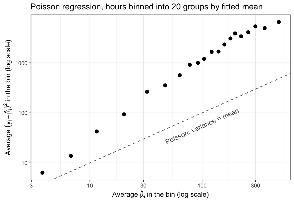
All 20 bins have an average squared residual above the dashed line. The average squared Pearson residual is \(\hat\phi = 11.3\): the hourly counts have about 11 times the variance around their fitted means that a Poisson distribution allows. The additive model’s \(\hat\phi\) is 25.6, so the hour-by-working-day features explained part of the excess variation, but \(\hat\phi\) remains far above \(1\).
The score equations involve \(y_i\) only through \(y_i - \mu_i\), never through its variance, so if the mean model is right \(\hat\beta\), the fitted means, and the rate ratios remain sensible estimates under overdispersion. The standard errors, computed as if the variance were \(\mu_i\), are too small, so \(z\)-statistics are too large and confidence intervals too narrow, and \(G^2\) is too large relative to its \(\chi^2_k\) reference. If \(Var[Y_i \mid x_i] = \phi\,\mu_i\), \(G^2\) is approximately \(\phi\,\chi^2_k\), so \(G^2/\hat\phi\) is approximately \(\chi^2_k\). For the bike counts \(G^2/\hat\phi = 11{,}380\), still 495 times its \(23\) degrees of freedom: the interaction test’s conclusion survives.
Overdispersion has two sources, as in the problems in logistic regression lecture: explanatory variables missing from the model that vary among observations with the same \(x_i\) (for the bike counts, plausibly conditions shared by the hours of one day), and events within one count that are not independent, such as riders who rent together. Adding features addresses only the first; the second falls under the remedies of the callout below.
NoteBeyond this course
Two standard remedies change the variance model rather than the mean model. Quasi-Poisson regression keeps \(\log \mu_i = x_i\beta\) and the estimates \(\hat\beta\) but assumes \(Var[Y_i \mid x_i] = \phi\,\mu_i\), estimating \(\phi\) by \(\hat\phi\) and multiplying every standard error by \(\sqrt{\hat\phi}\) (family = quasipoisson in glm()); deviance tests become \(F\)-tests. For the bike counts the factor is \(\sqrt{\hat\phi} = 3.36\), and the 95% interval for the rain/snow rate ratio widens from \((0.555, 0.564)\) to \((0.545, 0.575)\), still far from \(1\). Negative binomial regression replaces the Poisson with a distribution whose variance is \(\mu_i + \mu_i^2/\theta\) for an additional parameter \(\theta\), fit by maximum likelihood with MASS::glm.nb(). Neither is taught or tested here.
16.4 Conclusion
A generalized linear model has three components: a distribution for the response given the features, with mean \(\mu_i\); a linear predictor \(\eta_i = x_i\beta\), into which every feature-engineering device enters unchanged; and a link function with \(g(\mu_i) = \eta_i\), whose inverse keeps the mean in range. Linear, logistic, and Poisson regression pair the normal, Bernoulli, and Poisson distributions with the identity, logit, and log links, and variance functions \(1\), \(\mu(1-\mu)\), and \(\mu\).
Poisson regression models a count. Its mean \(e^{x_i\beta}\) is positive for every \(\beta\); \(e^{\beta_0}\) is the mean count when every feature is zero, and \(e^{\beta_j}\) a rate ratio, the factor multiplying the mean count per unit of feature \(j\) with the other features held fixed. A linear regression of \(\log Y_i\) also gives back-transformed fits that are positive and on which features act multiplicatively, but it requires every \(y_i > 0\) and models \(E[\log Y_i \mid x_i]\); its back-transformed fits estimate \(e^{E[\log Y_i \mid x_i]}\), which by Jensen’s inequality is at most the mean count \(E[Y_i \mid x_i]\). Poisson regression’s coefficients are maximum likelihood estimates; the score equations \(\sum_i x_{ij}(y_i - \mu_i) = 0\) have the logistic regression form, have no closed-form solution, and are solved by iteratively reweighted least squares. Inference uses the same Wald \(z\)-tests and intervals and the same drop-in-deviance test as logistic regression.
All of that inference assumes \(Var[Y_i \mid x_i] = \mu_i\). The average squared Pearson residual estimates the ratio of the actual variance to the mean; a value well above \(1\) signals overdispersion, under which the estimates remain usable if the mean model is right, but standard errors are too small, tests too liberal, and intervals too narrow.
The next lecture begins the resampling unit, ISLR2 Chapter 5: cross-validation estimates test error by repeatedly holding out part of the data, and uses those estimates to choose among models and flexibility settings.