19 Bootstrap

Learning objectives

After this lecture you should be able to

explain the bootstrap principle, that drawing $n$ observations with replacement from the sample imitates drawing new samples from the population, and compute a bootstrap standard error of a statistic with the bootstrap algorithm,
compare a bootstrap standard error with a formula-based standard error when one exists, such as the standard error of a regression coefficient from lm(), and explain why a bootstrap standard error is itself an estimate whose accuracy depends on the statistic and the sample size,
construct a percentile interval and a normal-approximation interval from a bootstrap distribution, and explain why the two differ when the bootstrap distribution is skewed or not centered at the estimate,
derive the probability $1 - (1 - 1/n)^n \approx 1 - 1/e \approx 0.632$ that a given observation appears in a bootstrap sample, and explain why it makes the bootstrap a poor estimator of test error, and
identify settings in which bootstrap standard errors and intervals are unreliable: small samples, heavy-tailed or skewed populations summarized by a mean-type statistic, extreme statistics such as the maximum, and dependent data.

19.1 Cloud seeding

19.1.1 Data

Question. Does seeding clouds with silver iodide increase rainfall, and by what factor?

Data. Sleuth3::case0301 records the volume of rainfall, in acre-feet, in a target area on 52 days suitable for cloud seeding. In a randomized experiment, the clouds were seeded on 26 of the days and left unseeded on the other 26. Each day is one observation.

The table gives each treatment’s number of days and the mean, geometric mean, median, standard deviation, minimum, and maximum of its rainfall, where the geometric mean is the exponential of the mean of log rainfall. The figure plots each day’s rainfall by treatment, with segments at each treatment’s mean (solid), geometric mean (dotted), and median (dashed); the second tab draws rainfall on a log scale.

Code

clouds <- case0301 |>
  mutate(Treatment = factor(Treatment, levels = c("Unseeded", "Seeded")),
         seeded = as.integer(Treatment == "Seeded"),
         # Horizontal jitter, computed once so that every figure below puts
         # each day in the same place.
         x_jit = as.integer(Treatment) + runif(n(), -0.15, 0.15))
n <- nrow(clouds)

cloud_summary <- clouds |>
  group_by(Treatment) |>
  summarize(days = n(), mean = mean(Rainfall),
            geo_mean = exp(mean(log(Rainfall))), median = median(Rainfall),
            sd = sd(Rainfall), min = min(Rainfall), max = max(Rainfall),
            sd_log = sd(log(Rainfall)), .groups = "drop")
summary_of <- function(trt, col) cloud_summary[[col]][cloud_summary$Treatment == trt]

cloud_table <- cloud_summary |>
  transmute(Treatment, days,
            across(c(mean, geo_mean, median, sd, min, max), \(v) fmt(v, 1))) |>
  knitr::kable(col.names = c("Treatment", "Days", "Mean", "Geometric mean",
                             "Median", "SD", "Min", "Max"),
               align = "lccccccc")

center_types <- c("Mean", "Geometric mean", "Median")
center_lines <- cloud_summary |>
  select(Treatment, Mean = mean, `Geometric mean` = geo_mean,
         Median = median) |>
  pivot_longer(-Treatment, names_to = "summary", values_to = "rainfall") |>
  mutate(x = as.integer(Treatment),
         summary = factor(summary, levels = center_types))

eda_plot <- ggplot(clouds, aes(x = x_jit, y = Rainfall)) +
  geom_point(aes(color = Treatment, shape = Treatment), size = 2) +
  geom_segment(data = center_lines,
               aes(x = x - 0.3, xend = x + 0.3, y = rainfall, yend = rainfall,
                   linetype = summary)) +
  scale_color_manual(values = treatment_colors) +
  scale_shape_manual(values = treatment_shapes) +
  scale_linetype_manual(values = c("Mean" = "solid",
                                   "Geometric mean" = "dotted",
                                   "Median" = "dashed")) +
  scale_x_continuous(breaks = 1:2, labels = levels(clouds$Treatment)) +
  labs(x = NULL, y = "Rainfall (acre-feet)", linetype = NULL,
       title = "Sleuth3::case0301, rainfall by treatment")

eda_plot_log <- eda_plot +
  scale_y_log10(labels = comma_labels) +
  labs(y = "Rainfall (acre-feet, log scale)")

Treatment	Days	Mean	Geometric mean	Median	SD	Min	Max
Unseeded	26	164.6	54.1	44.2	278.4	1.0	1,202.6
Seeded	26	442.0	169.7	221.6	650.8	4.1	2,745.6

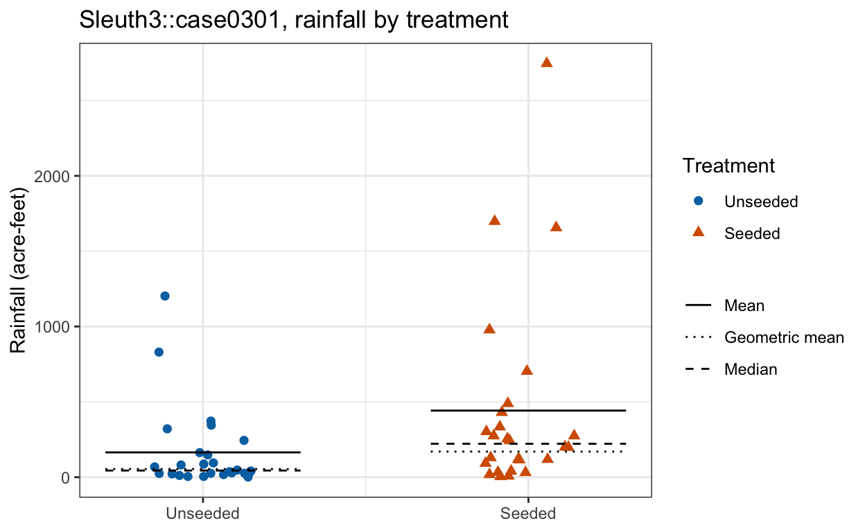
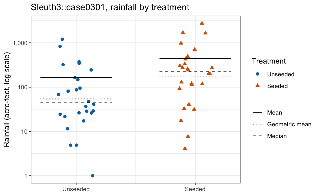
Both groups are strongly right-skewed: a few days with very large rainfall pull each mean far above its median, and the largest seeded day, 2,745.6 acre-feet, is more than 12 times the seeded median. On the log scale the two groups are roughly symmetric with similar spread (standard deviations of log rainfall 1.64 unseeded and 1.60 seeded), and on that axis each geometric mean lies close to its median. Seeded days tend to have more rainfall than unseeded days, though the two groups overlap heavily.

19.1.2 Multiplicative effect

The log-scale tab suggests modeling log rainfall as normal with a mean that depends on treatment,

\[\log Y_i = \beta_0 + \beta_1 D_i + \epsilon_i, \qquad \epsilon_i \stackrel{ind}{\sim} N\left(0, \sigma^2\right),\]

where

$Y_i$ is the rainfall on day $i$, in acre-feet,
$D_i = \mathrm{I}(\text{day } i \text{ seeded})$ is the indicator of seeding,
$\beta_0$ is the mean log rainfall on unseeded days,
$\beta_1$ is the difference in mean log rainfall, seeded minus unseeded, and
$\sigma^2$ is the variance of log rainfall about its treatment mean.

Adding $\beta_1$ to log rainfall multiplies rainfall by $e^{\beta_1}$, so the effect of seeding is the factor

\[\theta = e^{\beta_1}, \qquad \hat\theta = e^{\hat\beta_1} = \frac{\tilde y_S}{\tilde y_U},\]

where

$\theta$ is the factor by which seeding multiplies median rainfall, since under the model the median of $Y_i$ is $e^{\beta_0 + \beta_1 D_i}$,
$\hat\beta_1 = \overline{\log y}_S - \overline{\log y}_U$ is the least squares estimate of $\beta_1$, the difference between the sample means of log rainfall on seeded and unseeded days, and
$\tilde y_S = \exp\left(\overline{\log y}_S\right)$ and $\tilde y_U = \exp\left(\overline{\log y}_U\right)$ are the sample geometric means of rainfall on seeded and unseeded days, so that $\hat\theta$ is their ratio.

Throughout this chapter $\theta$ is the quantity whose standard error is wanted and $\hat\theta$ its estimate; for the cloud data, $\theta = e^{\beta_1}$.

cloud_lm <- lm(log(Rainfall) ~ seeded, data = clouds)
summary(cloud_lm)$coefficients

            Estimate Std. Error   t value     Pr(>|t|)
(Intercept) 3.990406  0.3178687 12.553628 4.481375e-17
seeded      1.143781  0.4495342  2.544369 1.408266e-02

theta_hat <- exp(coef(cloud_lm)[["seeded"]])
theta_hat

[1] 3.138614

The estimated mean log rainfall on unseeded days is $\hat\beta_0 = 3.99$, a geometric mean of $e^{\hat\beta_0} = 54.1$ acre-feet. Seeded days averaged $\hat\beta_1 = 1.14$ more log rainfall, with standard error 0.45, so seeding multiplied the geometric mean rainfall by $\hat\theta = 3.14$. lm() reports a standard error for $\hat\beta_1$ but none for $\hat\theta$, the number that answers the question.

19.2 Standard error

19.2.1 Sampling distribution

Repeating the experiment on 52 new days would give different rainfall and a different $\hat\theta$. Before the data are collected, $\hat\theta$ is a random variable, and its distribution over repeated samples from the population is its sampling distribution. The standard error of $\hat\theta$ is the standard deviation of that distribution,

\[\text{SE}(\hat\theta) = \sqrt{Var\left[\hat\theta\right]}.\]

Simulating the sampling distribution would mean running the experiment again and again, which requires access to the population.

19.2.2 Formulas

For some statistics, probability theory gives the standard error as a function of population quantities that the sample can estimate. The sample mean of $n$ independent observations with standard deviation $\sigma$ has $\text{SE}(\bar y) = \sigma/\sqrt n$, estimated by $s/\sqrt n$, and lm() reports the standard error of each regression coefficient. The estimate $\hat\theta = e^{\hat\beta_1}$ is a nonlinear function of a coefficient, and no column of the lm() output gives its standard error. A median, a quantile, and the AUC of a fitted classifier have no simple standard-error formula either, and a statistic computed by an algorithm rather than a formula often has none at all.

19.3 Bootstrap

19.3.1 Resampling

The first tab below repeats the 52 days on the log scale. Each later tab draws 52 days with replacement from those 52, so that a day can be drawn more than once or not at all. Filled points are days that were drawn, larger the more times they were drawn, open grey points are days that were not drawn, and the solid segments mark each treatment’s geometric mean rainfall in that sample. Each title gives the sample’s ratio of geometric means.

Code

# Draw three illustrative bootstrap samples and record how many times each
# day was drawn.
illustrative_counts <- map(1:3, \(b) tabulate(sample(n, replace = TRUE),
                                              nbins = n))
# One size scale for every tab, so a point's size means the same thing in each.
max_count <- max(unlist(illustrative_counts))

resample_plot <- function(counts, title) {
  d <- clouds |> mutate(count = counts)
  drawn   <- filter(d, count > 0)
  undrawn <- filter(d, count == 0)
  group_geo_means <- drawn |>
    group_by(Treatment) |>
    summarize(rainfall = exp(weighted.mean(log(Rainfall), count)),
              .groups = "drop") |>
    mutate(x = as.integer(Treatment))
  ratio <- group_geo_means$rainfall[2] / group_geo_means$rainfall[1]

  ggplot(drawn, aes(x = x_jit, y = Rainfall)) +
    geom_point(data = undrawn, color = "grey60",
               shape = ifelse(undrawn$Treatment == "Seeded", 2, 1), size = 2) +
    geom_point(aes(color = Treatment, shape = Treatment, size = count)) +
    geom_segment(data = group_geo_means,
                 aes(x = x - 0.3, xend = x + 0.3, y = rainfall,
                     yend = rainfall)) +
    scale_color_manual(values = treatment_colors) +
    scale_shape_manual(values = treatment_shapes) +
    scale_size_area(max_size = 5, breaks = 1:max_count,
                    limits = c(0, max_count)) +
    scale_x_continuous(breaks = 1:2, labels = levels(clouds$Treatment),
                       limits = c(0.6, 2.4)) +
    scale_y_log10(labels = comma_labels) +
    labs(x = NULL, y = "Rainfall (acre-feet, log scale)",
         size = "Times drawn",
         title = sprintf("%s: ratio of geometric means = %.2f", title, ratio))
}

original_plot <- resample_plot(rep(1, n), "Original sample")
resample_plots <- imap(illustrative_counts,
                       \(cnt, b) resample_plot(cnt, paste("Bootstrap sample", b)))
n_distinct_illustrative <- map_int(illustrative_counts, \(cnt) sum(cnt > 0))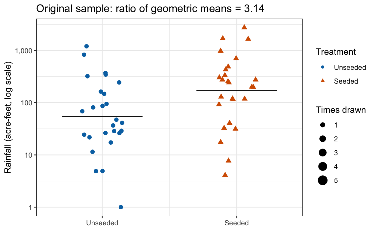

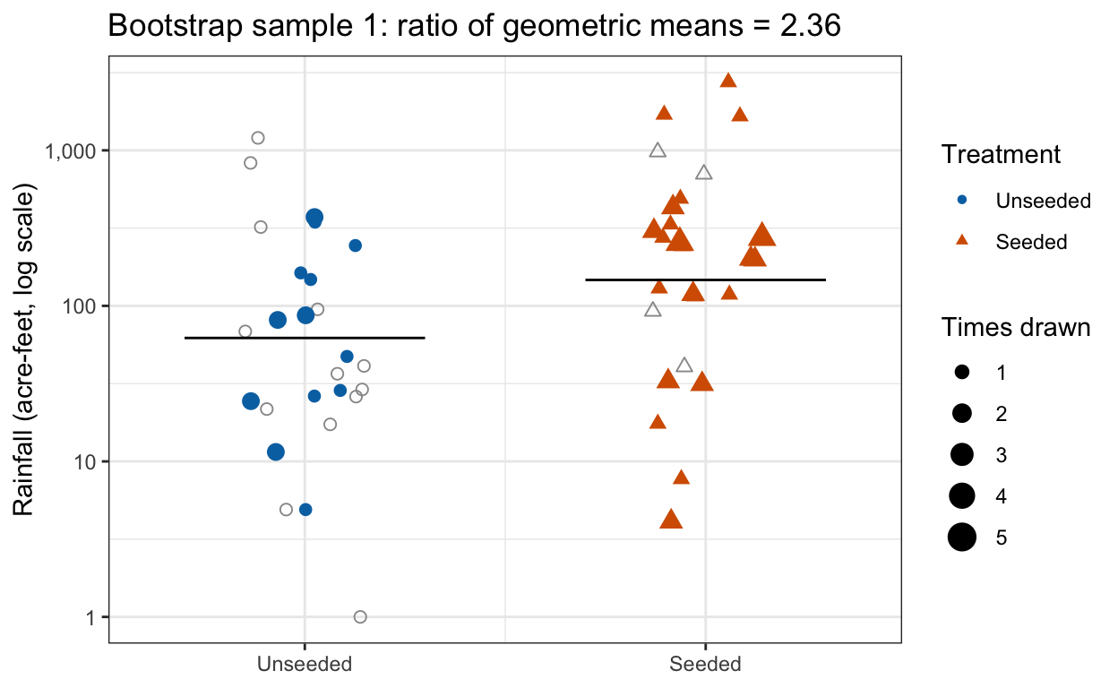
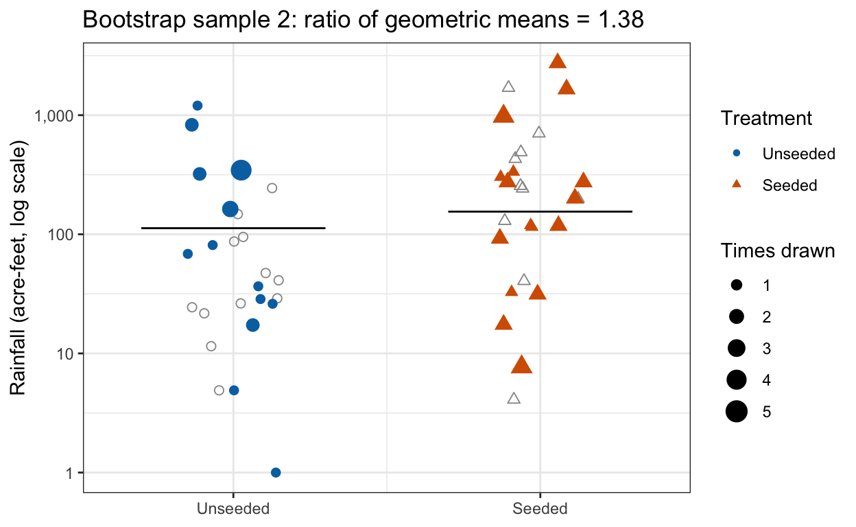
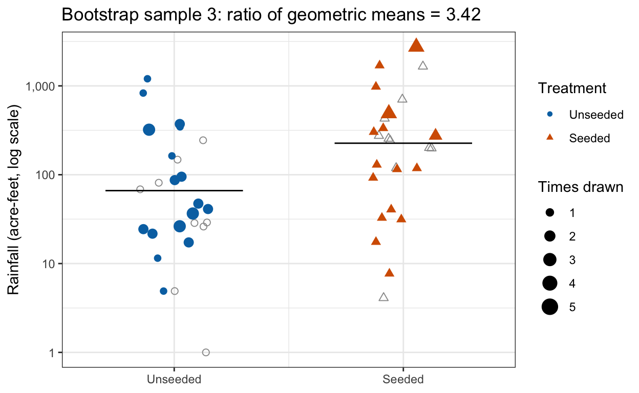
The three resamples contain 35, 30, and 33 of the 52 days, each with some days repeated, and their ratios of geometric means differ from one another and from $\hat\theta = 3.14$.

This is the bootstrap: it treats the sample as if it were the population. The population of all suitable days is unavailable, but the 52 observed days are, and drawing 52 days with replacement from them imitates running the experiment again. Each resample is a bootstrap sample, and how much the statistic varies across bootstrap samples estimates how much $\hat\theta$ varies across experiments.

19.3.2 Algorithm

Write the data set of $n$ observations as $Z$ (here 52 days, each a rainfall and a treatment). The bootstrap standard error of a statistic $\hat\theta$ computed from $Z$ is found in three steps.

For $b = 1, \ldots, B$, draw a bootstrap sample $Z^{*b}$ of $n$ observations from $Z$ with replacement, each draw choosing each observation with probability $1/n$.
Compute the statistic on each bootstrap sample, exactly as $\hat\theta$ was computed on $Z$, giving $\hat\theta^{*1}, \ldots, \hat\theta^{*B}$.
Take their standard deviation,

\[\text{SE}_B(\hat\theta) = \sqrt{\frac{1}{B-1}\sum_{b=1}^B \left(\hat\theta^{*b} - \bar\theta^{*}\right)^2}, \qquad \bar\theta^{*} = \frac{1}{B}\sum_{b=1}^B \hat\theta^{*b},\]

where

$B$ is the number of bootstrap samples, chosen by the analyst (a few thousand is typical),
$\hat\theta^{*b}$ is the statistic computed on bootstrap sample $b$,
$\bar\theta^{*}$ is the mean of the $B$ bootstrap statistics, and
$\text{SE}_B(\hat\theta)$ is the bootstrap standard error of $\hat\theta$.

The $B$ values $\hat\theta^{*b}$ form the bootstrap distribution of $\hat\theta$. In R, step 1 is sample(n, replace = TRUE), which returns the row numbers of one bootstrap sample. It draws the 52 days without regard to treatment, so the numbers of seeded and unseeded days vary from one bootstrap sample to the next. Step 2 refits the regression and exponentiates its slope; the loop also keeps the slope $\hat\beta_1^{*b}$ itself, used in the next subsection.

B <- 2000
boot <- tibble(b = 1:B) |>
  mutate(
    i     = map(b, \(b) sample(n, replace = TRUE)),                 # step 1
    slope = map_dbl(i, \(i) coef(lm(log(Rainfall) ~ seeded,
                                    data = clouds[i, ]))[["seeded"]]),
    theta = exp(slope)                                              # step 2
  )
se_boot_theta <- sd(boot$theta)                                     # step 3
se_boot_theta

[1] 1.554263

The histogram shows the 2,000 values of $\hat\theta^{*b}$, with a solid line at $\hat\theta$.

Code

boot_hist_plot <- ggplot(boot, aes(x = theta)) +
  geom_histogram(bins = 50, fill = "grey75", color = "grey45") +
  geom_vline(xintercept = theta_hat, linewidth = 0.9) +
  labs(x = expression("Bootstrap ratio of geometric means, " *
                        hat(theta)^"*b"),
       y = "Bootstrap samples",
       title = "Bootstrap distribution of the ratio of geometric means")
boot_theta_range <- range(boot$theta)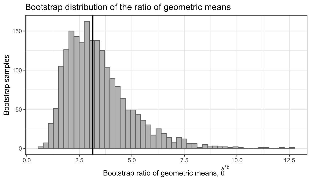

The bootstrap distribution is right-skewed, running from 0.66 to 12.62. Its standard deviation is the bootstrap standard error, $\text{SE}_B(\hat\theta) = 1.55$.

19.3.3 Regression slope

Where a formula exists, the bootstrap should agree with it. The slope $\hat\beta_1$ has the standard error lm() reported, and the loop above recorded $\hat\beta_1^{*b}$ on each bootstrap sample. The histogram shows those 2,000 bootstrap slopes on the density scale, with the normal density centered at $\hat\beta_1$ with the lm() standard error drawn as a dashed curve.

Code

se_boot_slope <- sd(boot$slope)
slope_grid <- tibble(slope = seq(min(boot$slope), max(boot$slope),
                                 length.out = 400)) |>
  mutate(density = dnorm(slope, b_lm[["seeded"]], se_lm[["seeded"]]))

slope_plot <- ggplot(boot, aes(x = slope)) +
  geom_histogram(aes(y = after_stat(density)), bins = 50,
                 fill = "grey75", color = "grey45") +
  geom_line(data = slope_grid, aes(y = density), linetype = "dashed",
            linewidth = 0.9) +
  geom_vline(xintercept = b_lm[["seeded"]], linewidth = 0.9) +
  labs(x = expression("Bootstrap slope, " * hat(beta)[1]^"*b" *
                        " (difference in mean log rainfall)"),
       y = "Density",
       title = "Bootstrap slopes and the normal density from lm()")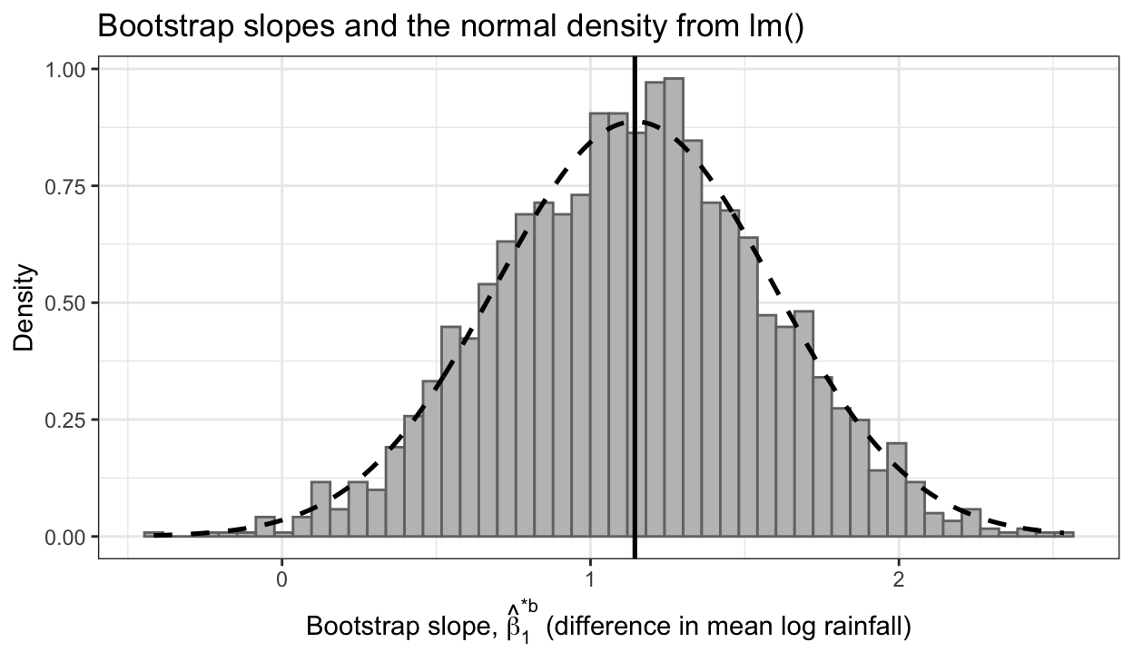

The bootstrap standard error of the slope is $\text{SE}_B(\hat\beta_1) = 0.437$, against 0.450 from lm(), and the histogram follows the normal curve. Each $\hat\theta^{*b}$ is $e^{\hat\beta_1^{*b}}$, so the right skew of the $\hat\theta^{*b}$ histogram is this bell shape passed through the exponential function.

19.3.4 Known population

Whether the bootstrap distribution of $\hat\theta$ imitates its sampling distribution can only be checked where the sampling distribution is known, so this subsection simulates experiments from a known population: the log-scale regression model with $\beta_0$, $\beta_1$, and $\sigma$ set to the cloud data’s estimates $\hat\beta_0 = 3.99$, $\hat\beta_1 = 1.14$, and $\hat\sigma = 1.62$. For this population $\theta = e^{\beta_1} = 3.14$.

The simulation runs the experiment, 26 unseeded and 26 seeded days, many times to obtain the sampling distribution of $\hat\theta$. It then runs one more experiment, treats it as the only sample available, and bootstraps it 2,000 times, resampling all its days together as for the cloud data. The first tab shows the sampling distribution, with a solid line at $\theta$; the second shows the bootstrap distribution from the one experiment, with a solid line at that experiment’s $\hat\theta$. Both use the same horizontal axis, cut at the 99.9th percentile of the simulated values.

Code

pop <- list(beta0 = b_lm[["(Intercept)"]], beta1 = b_lm[["seeded"]],
            sigma = sigma(cloud_lm))
theta_pop <- exp(pop$beta1)

# R simulated experiments with m days per treatment, as an m-row matrix of
# unseeded log rainfall and an m-row matrix of seeded log rainfall, one column
# per experiment.
draw_experiments <- function(m, R) {
  list(U = matrix(rnorm(m * R, pop$beta0, pop$sigma), m, R),
       S = matrix(rnorm(m * R, pop$beta0 + pop$beta1, pop$sigma), m, R))
}
# Every statistic in this chapter, for each column (experiment): the slope
# (difference in mean log rainfall, the least squares slope), theta-hat, and
# the ratio of mean rainfall (used under Limitations).
experiment_stats <- function(x) {
  slope <- colMeans(x$S) - colMeans(x$U)
  tibble(slope = slope, theta = exp(slope),
         ratio = colMeans(exp(x$S)) / colMeans(exp(x$U)))
}
# B bootstrap samples of one data set (rainfall y, seeding indicator s), all at
# once: column b of idx holds the row numbers of bootstrap sample b, drawn from
# all the days together as in the cloud bootstrap.
bootstrap_stats <- function(y, s, B) {
  N <- length(y)
  idx <- matrix(sample.int(N, N * B, replace = TRUE), N, B)
  Y <- matrix(y[idx], N, B)
  S <- matrix(s[idx], N, B)
  n_S <- colSums(S)
  slope <- colSums(log(Y) * S) / n_S - colSums(log(Y) * (1 - S)) / (N - n_S)
  tibble(slope = slope, theta = exp(slope),
         ratio = (colSums(Y * S) / n_S) / (colSums(Y * (1 - S)) / (N - n_S)))
}

# Statistics for R experiments, simulated in batches of 10,000 to limit memory.
simulate_stats <- function(m, R, batch = 10000) {
  map(seq_len(R / batch), \(k) experiment_stats(draw_experiments(m, batch))) |>
    list_rbind()
}

# The ratio of means has a heavy-tailed sampling distribution, so its standard
# deviation needs many experiments to pin down: 10,000 can be off by over 10%.
n_experiments <- 100000
m_cloud <- sum(clouds$seeded == 1)   # 26 days per treatment
sampling <- simulate_stats(m_cloud, n_experiments)
se_true <- map_dbl(sampling, sd)
# se_true is itself a simulation estimate. Its Monte Carlo standard error, from
# the spread of the standard deviations of 20 equal batches of experiments, is
# reported relative to se_true.
se_true_mcse <- map_dbl(sampling, \(v) {
  sd(tapply(v, rep(1:20, each = n_experiments / 20), sd)) / sqrt(20) / sd(v)
})

one_experiment <- draw_experiments(m_cloud, 1)
one_y <- exp(c(one_experiment$U, one_experiment$S))
one_s <- rep(0:1, each = m_cloud)
theta_hat_one <- experiment_stats(one_experiment)$theta
one_boot      <- bootstrap_stats(one_y, one_s, B)$theta
se_boot_one   <- sd(one_boot)

# A shared axis from 0 to the 99.9th percentile of the simulated values; the
# few experiments beyond it would otherwise squeeze the histograms flat.
x_limits <- c(0, quantile(c(sampling$theta, one_boot), 0.999))
known_hist <- function(values, line_at, title) {
  ggplot(tibble(value = values), aes(x = value)) +
    geom_histogram(aes(y = after_stat(density)), boundary = 0,
                   binwidth = diff(x_limits) / 60,
                   fill = "grey75", color = "grey45") +
    geom_vline(xintercept = line_at, linewidth = 0.9) +
    coord_cartesian(xlim = x_limits) +
    labs(x = "Ratio of geometric means", y = "Density", title = title)
}
sampling_plot <- known_hist(
  sampling$theta, theta_pop,
  sprintf("Sampling distribution: %s experiments, SE = %.2f",
          fmt(n_experiments), se_true[["theta"]]))
one_boot_plot <- known_hist(
  one_boot, theta_hat_one,
  sprintf("Bootstrap distribution: one experiment, SE_B = %.2f", se_boot_one))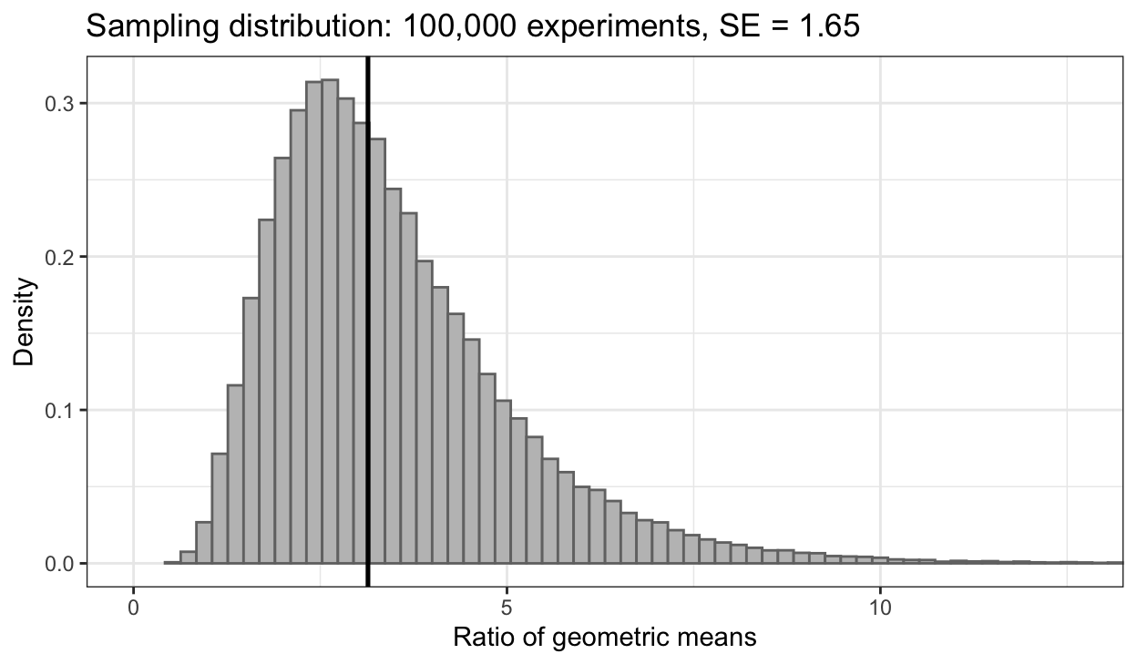

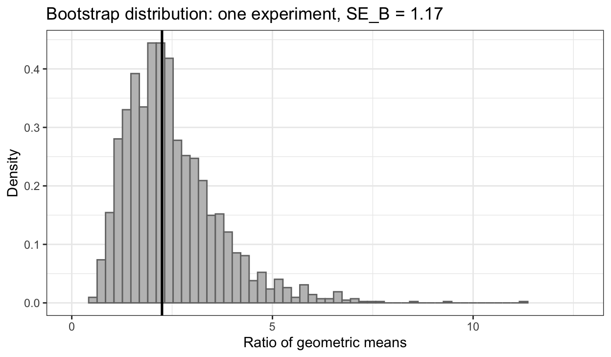
Both distributions are right-skewed. Over 100,000 experiments, $\hat\theta$ has standard error 1.65 (a simulation estimate, accurate to about $$1%, two Monte Carlo standard errors). The bootstrap distribution is centered at that experiment’s $\hat\theta = 2.25$, not at $\theta = 3.14$: it estimates the spread and shape of the sampling distribution, not the location of $\theta$. Its standard deviation, $\text{SE}_B(\hat\theta) = 1.17$, is 0.71 times the true standard error, and that experiment’s $\hat\theta$ is 0.72 times $\theta$. The next subsection shows that these two ratios tend to move together.

19.3.5 Accuracy

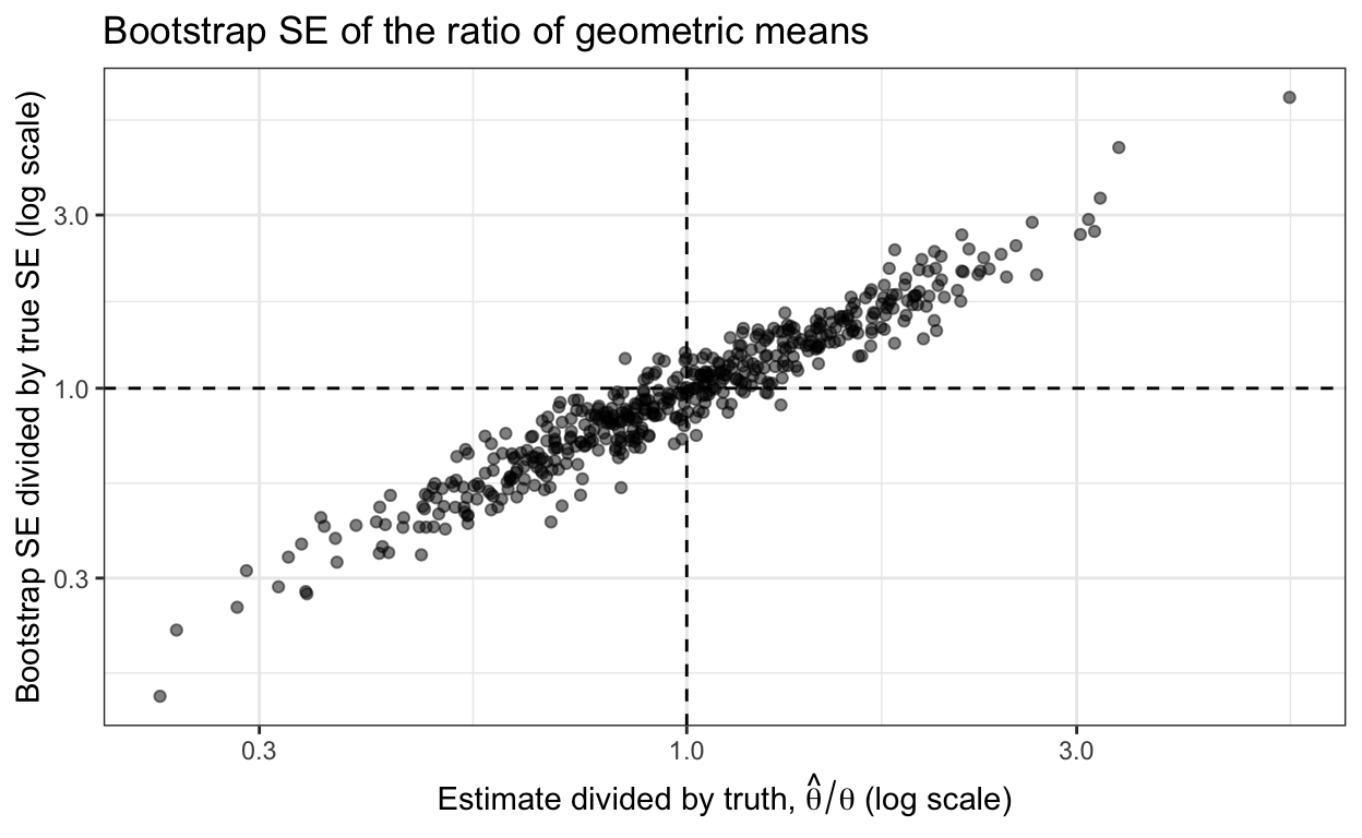
A bootstrap standard error is itself an estimate, computed from one sample, and a different sample gives a different value. To see how far it typically lands from the truth, the simulation bootstraps 500 further experiments of 26 days per treatment, 1,000 times each, and divides each experiment’s $\text{SE}_B$ by the true standard error. The first tab shows these ratios for the slope $\hat\beta_1$ and for $\hat\theta$; the second plots, for each experiment, the ratio for $\hat\theta$ against how far that experiment’s $\hat\theta$ fell from $\theta$.

Code

# Bootstrap n_check simulated experiments with m days per treatment. Each row
# holds one experiment's estimates, its bootstrap SEs, and its 95% percentile
# and normal-approximation intervals for theta.
check_experiments <- function(m, n_check, B_check) {
  map(1:n_check, \(r) {
    x <- draw_experiments(m, 1)
    est <- experiment_stats(x)
    bs <- bootstrap_stats(exp(c(x$U, x$S)), rep(0:1, each = m), B_check)
    tibble(m = m, theta_hat = est$theta,
           se_b_slope = sd(bs$slope), se_b_theta = sd(bs$theta),
           se_b_ratio = sd(bs$ratio),
           perc_lo = quantile(bs$theta, 0.025),
           perc_hi = quantile(bs$theta, 0.975),
           norm_lo = est$theta - qnorm(0.975) * sd(bs$theta),
           norm_hi = est$theta + qnorm(0.975) * sd(bs$theta))
  }) |> list_rbind()
}
checks <- check_experiments(m_cloud, n_check, B_check) |>
  mutate(rel_slope = se_b_slope / se_true[["slope"]],
         rel_theta = se_b_theta / se_true[["theta"]])

# Typical relative error: the median of |SE_B / SE - 1| over experiments.
typical_error <- c(slope = median(abs(checks$rel_slope - 1)),
                   theta = median(abs(checks$rel_theta - 1)))
median_rel    <- c(slope = median(checks$rel_slope),
                   theta = median(checks$rel_theta))
slope_within  <- mean(abs(checks$rel_slope - 1) <= 0.10)

accuracy_labels <- c(rel_slope = "Slope, difference in mean log rainfall",
                     rel_theta = "Ratio of geometric means")
accuracy_long <- checks |>
  select(rel_slope, rel_theta) |>
  pivot_longer(everything(), names_to = "stat", values_to = "relative") |>
  mutate(stat = factor(accuracy_labels[stat], levels = accuracy_labels))
accuracy_plot <- ggplot(accuracy_long, aes(x = relative)) +
  geom_histogram(bins = 40, fill = "grey75", color = "grey45") +
  geom_vline(xintercept = 1, linewidth = 0.9) +
  scale_x_log10() +
  facet_wrap(~ stat, ncol = 1) +
  labs(x = "Bootstrap SE divided by true SE (log scale)",
       y = "Simulated experiments",
       title = sprintf("%d simulated experiments, %d days per treatment",
                       n_check, m_cloud))

accuracy_scatter <- ggplot(checks, aes(x = theta_hat / theta_pop,
                                       y = rel_theta)) +
  geom_hline(yintercept = 1, linetype = "dashed") +
  geom_vline(xintercept = 1, linetype = "dashed") +
  geom_point(alpha = 0.5) +
  scale_x_log10() +
  scale_y_log10() +
  labs(x = expression("Estimate divided by truth, " * hat(theta) / theta *
                        " (log scale)"),
       y = "Bootstrap SE divided by true SE (log scale)",
       title = "Bootstrap SE of the ratio of geometric means")
scatter_cor <- cor(log(checks$theta_hat), log(checks$rel_theta))

coverage <- checks |>
  summarize(perc = mean(perc_lo < theta_pop & theta_pop < perc_hi),
            perc_above = mean(perc_hi < theta_pop),
            perc_below = mean(perc_lo > theta_pop),
            norm = mean(norm_lo < theta_pop & theta_pop < norm_hi),
            norm_above = mean(norm_hi < theta_pop),
            norm_below = mean(norm_lo > theta_pop),
            norm_negative = mean(norm_lo < 0))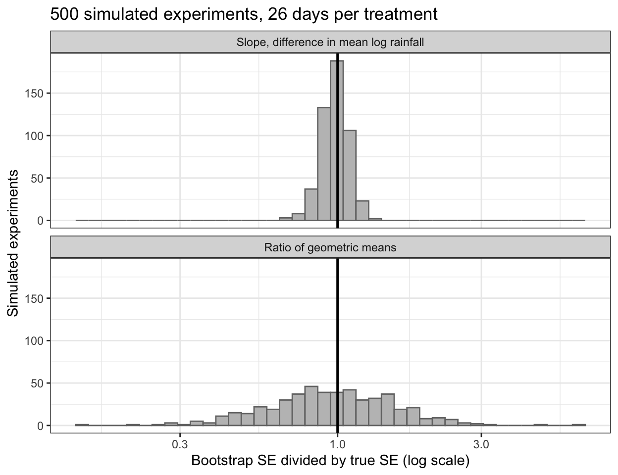

For the slope, $\text{SE}_B$ is typically within 6% of the true standard error (the median of $|\text{SE}_B/\text{SE} - 1|$ over the experiments), and within 10% in 69% of them. For $\hat\theta$ the median ratio is 0.96, so $\text{SE}_B$ is not systematically too small or too large, but its typical error is 31%.

The second tab shows where that error comes from: experiments whose $\hat\theta$ overshoots $\theta$ also overstate its standard error (correlation 0.96 on the log scales). Each bootstrap statistic is $\hat\theta^{*b} = \hat\theta\, e^{\hat\beta_1^{*b} - \hat\beta_1}$, so

\[\text{SE}_B(\hat\theta) = \hat\theta \times \text{SD}_B\left(e^{\hat\beta_1^{*b} - \hat\beta_1}\right),\]

where

$\text{SD}_B(\cdot)$ is the standard deviation over the $B$ bootstrap samples, and
the second factor depends only on the spread of the bootstrap slopes, which the bootstrap estimates as well as it estimates $\text{SE}(\hat\beta_1)$.

The first factor is $\hat\theta$ itself. The standard error of $\hat\theta$ is proportional to $\theta$, which is known only through $\hat\theta$, so no estimate of $\text{SE}(\hat\theta)$, bootstrap or formula, can be much more accurate than $\hat\theta$. For the cloud data, $\text{SE}_B(\hat\theta) = 1.55$ is best read as “about 1.6, give or take 31%.”

19.4 Confidence intervals

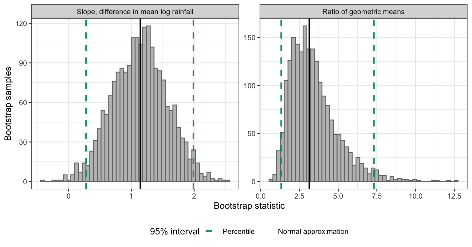
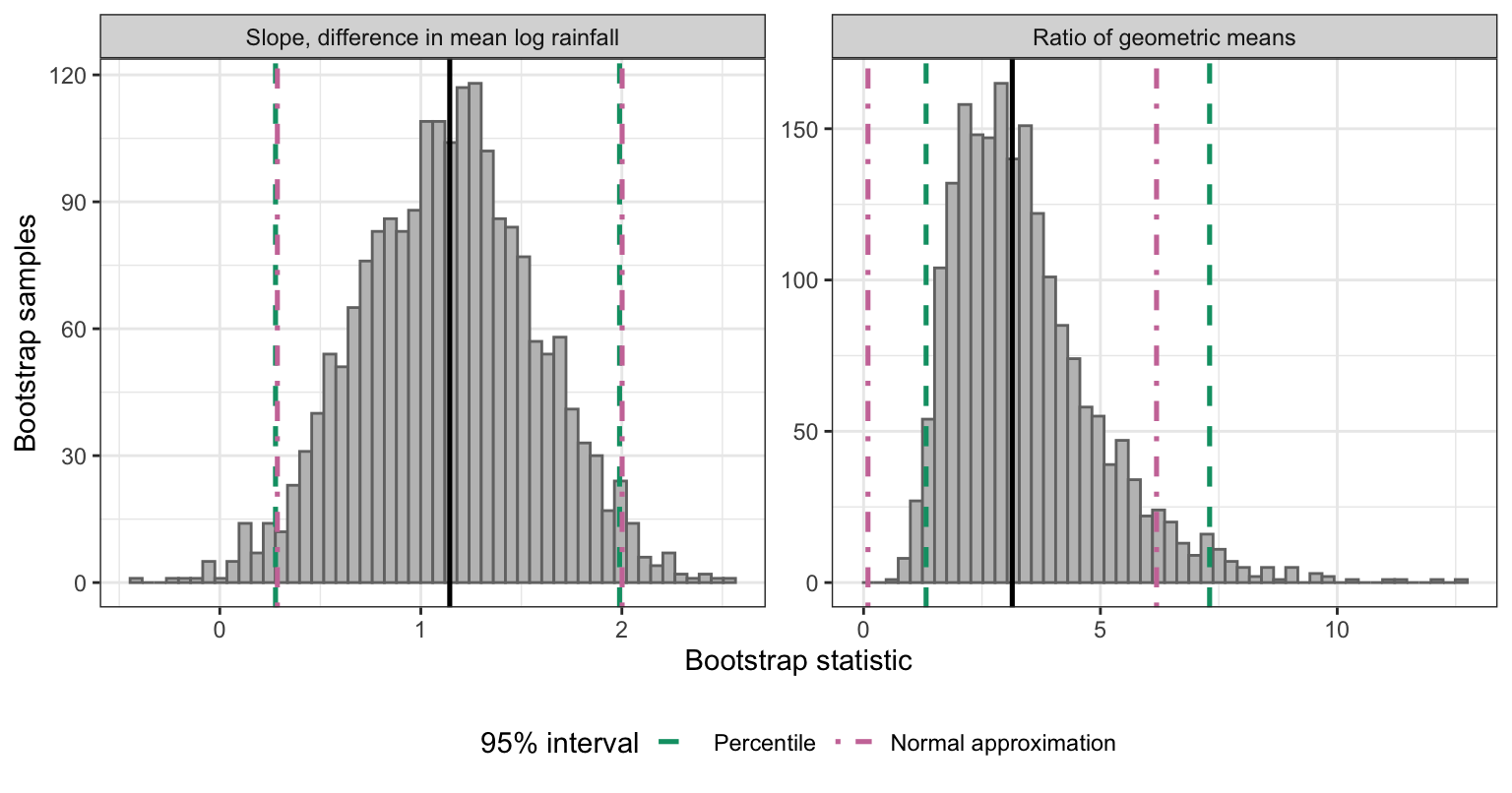
A standard error describes the spread of a statistic; a confidence interval uses the whole bootstrap distribution. The first tab shows the bootstrap distributions of the slope, $\hat\beta_1^{*b}$, and the ratio of geometric means, $\hat\theta^{*b}$, each with a solid line at the original estimate. The second tab adds each statistic’s 95% percentile interval as dashed lines, and the third adds its 95% normal-approximation interval as dot-dashed lines; both intervals are defined below the figure.

Code

alpha <- 0.05
z <- qnorm(1 - alpha / 2)
stat_labels <- c(slope = "Slope, difference in mean log rainfall",
                 theta = "Ratio of geometric means")
estimates <- c(slope = b_lm[["seeded"]], theta = theta_hat)
se_boot   <- c(slope = se_boot_slope, theta = se_boot_theta)

intervals <- tibble(stat = names(estimates), estimate = estimates,
                    se = se_boot) |>
  mutate(perc_lo = map_dbl(stat, \(s) quantile(boot[[s]], alpha / 2)),
         perc_hi = map_dbl(stat, \(s) quantile(boot[[s]], 1 - alpha / 2)),
         norm_lo = estimate - z * se,
         norm_hi = estimate + z * se,
         # The t interval for the slope from lm(), and its exponential for
         # theta.
         lm_lo = if_else(stat == "slope", ci_lm[[1]], exp(ci_lm[[1]])),
         lm_hi = if_else(stat == "slope", ci_lm[[2]], exp(ci_lm[[2]])))
interval_of <- function(s, col) intervals[[col]][intervals$stat == s]

boot_long <- boot |>
  select(slope, theta) |>
  pivot_longer(everything(), names_to = "stat") |>
  mutate(stat = factor(stat_labels[stat], levels = stat_labels))
estimate_lines <- tibble(stat = factor(stat_labels[names(estimates)],
                                       levels = stat_labels),
                         value = estimates)
interval_lines_df <- intervals |>
  pivot_longer(c(perc_lo, perc_hi, norm_lo, norm_hi),
               names_to = c("method", "end"), names_sep = "_") |>
  mutate(method = if_else(method == "perc", "Percentile",
                          "Normal approximation"),
         method = factor(method, levels = names(interval_colors)),
         stat = factor(stat_labels[stat], levels = stat_labels))

interval_base <- ggplot(boot_long, aes(x = value)) +
  geom_histogram(bins = 50, fill = "grey75", color = "grey45") +
  geom_vline(data = estimate_lines, aes(xintercept = value),
             linewidth = 0.9) +
  facet_wrap(~ stat, scales = "free") +
  labs(x = "Bootstrap statistic", y = "Bootstrap samples")
interval_layer <- function(methods) {
  list(
    geom_vline(data = filter(interval_lines_df, method %in% methods),
               aes(xintercept = value, color = method, linetype = method),
               linewidth = 0.9, key_glyph = "path"),
    scale_color_manual(values = interval_colors, drop = FALSE),
    scale_linetype_manual(values = interval_lines, drop = FALSE),
    labs(color = "95% interval", linetype = "95% interval"),
    theme(legend.position = "bottom")
  )
}
interval_plot_0 <- interval_base
interval_plot_1 <- interval_base + interval_layer("Percentile")
interval_plot_2 <- interval_base + interval_layer(names(interval_colors))

interval_text <- function(lo, hi) sprintf("(%s, %s)", fmt(lo, 2), fmt(hi, 2))
interval_table <- intervals |>
  mutate(Statistic = stat_labels[stat],
         Estimate = fmt(estimate, 2),
         `Bootstrap SE` = fmt(se, 2),
         Percentile = interval_text(perc_lo, perc_hi),
         `Normal approximation` = interval_text(norm_lo, norm_hi),
         `From lm()` = interval_text(lm_lo, lm_hi)) |>
  select(Statistic, Estimate, `Bootstrap SE`, Percentile,
         `Normal approximation`, `From lm()`) |>
  knitr::kable(align = "lccccc")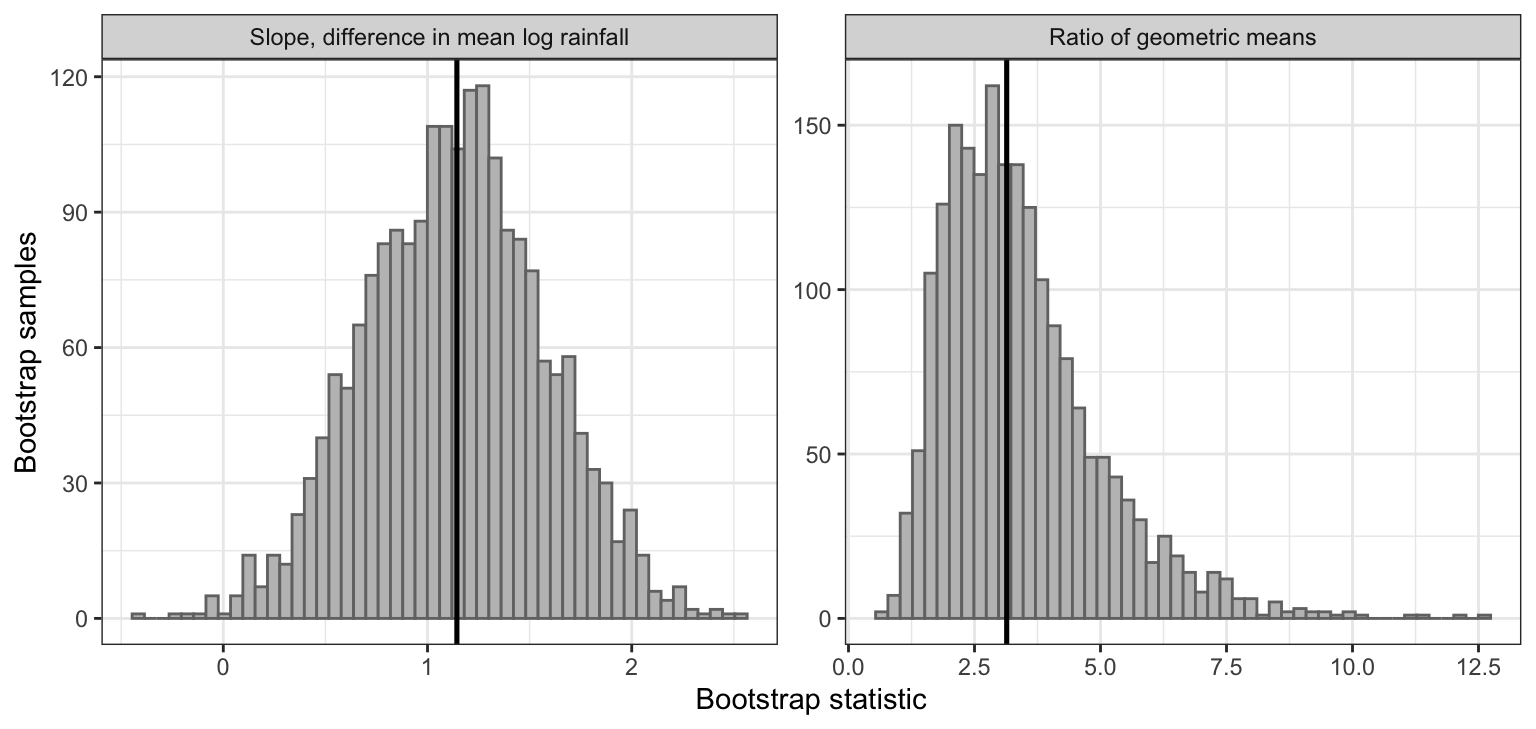

19.4.1 Percentile interval

If some monotone transformation of $\hat\theta$ has an approximately normal sampling distribution, as $\log\hat\theta = \hat\beta_1$ does here, the middle $1 - \alpha$ of the bootstrap distribution gives a range of plausible values of $\theta$, without the transformation having to be known. The $(1 - \alpha)100\%$ percentile interval is

\[\left(\hat\theta^{*}_{(\alpha/2)},\ \hat\theta^{*}_{(1-\alpha/2)}\right),\]

where $\hat\theta^{*}_{(q)}$ is the $q$ quantile of the $B$ bootstrap statistics $\hat\theta^{*1}, \ldots, \hat\theta^{*B}$. In R it is quantile(boot$theta, c(0.025, 0.975)) for a 95% interval.

For the ratio of geometric means the 95% percentile interval is (1.32, 7.30).

For example,

A percentile interval moves with a monotone transformation of the statistic. Since $\hat\theta^{*b} = e^{\hat\beta_1^{*b}}$, the quantiles of the $\hat\theta^{*b}$ are the exponentials of the quantiles of the $\hat\beta_1^{*b}$. The 95% percentile interval for $\beta_1$ is (0.277, 1.989), and its exponential, (1.32, 7.30), is the percentile interval for $\theta$ above. A normal-approximation interval does not move this way: exponentiating the one for $\beta_1$ does not give the one for $\theta$.

19.4.2 Normal-approximation interval

If the sampling distribution of $\hat\theta$ is approximately normal, the usual form of interval applies with the bootstrap standard error,

\[\hat\theta \pm z_{1-\alpha/2}\,\text{SE}_B(\hat\theta),\]

where $z_{1-\alpha/2}$ is the $(1 - \alpha/2)$ quantile of the standard normal distribution, 1.96 for a 95% interval.

For the ratio of geometric means the 95% normal-approximation interval is (0.09, 6.18).

19.4.3 Comparison

The table collects both intervals for both statistics. Its last column is the $t$ interval from lm() for $\beta_1$ and, for $\theta$, the exponential of that interval.

Statistic	Estimate	Bootstrap SE	Percentile	Normal approximation	From lm()
Slope, difference in mean log rainfall	1.14	0.44	(0.28, 1.99)	(0.29, 2.00)	(0.24, 2.05)
Ratio of geometric means	3.14	1.55	(1.32, 7.30)	(0.09, 6.18)	(1.27, 7.74)

For the slope the three intervals nearly coincide: each endpoint differs from the $t$ interval’s by at most 0.06, because the bootstrap distribution of $\hat\beta_1^{*b}$ is close to normal and centered at $\hat\beta_1$. For the ratio of geometric means the two bootstrap intervals differ. The normal-approximation interval is symmetric about $\hat\theta$, and its lower limit, 0.09, lies below every bootstrap value. The percentile interval follows the skew: its upper limit is 4.17 above $\hat\theta$ and its lower limit 1.82 below it, like the exponentiated $t$ interval (1.27, 7.74).

The two intervals agree when the bootstrap distribution is approximately normal and centered at $\hat\theta$. Skewness separates them, and so does bias, a bootstrap distribution centered away from $\hat\theta$, which shifts the percentile interval but not the normal-approximation interval.

In the 500 simulated experiments of the Accuracy subsection, the 95% percentile interval contained $\theta$ in 93.6% of them, missing low (entirely below $\theta$) in 3.6% and high in 2.8%. The normal-approximation interval contained $\theta$ in 93.2%, missing low in 6.8% and high in 0.0%, and its lower limit was negative, a value no ratio of positive quantities can take, in 51.0%. Both cover $\theta$ at close to the nominal rate, but only the percentile interval stays within the possible values of $\theta$ and splits its misses between the two sides.

19.5 Sample overlap

The bootstrap samples in the Resampling tabs each left out some of the 52 days. The bar chart counts, over all 2,000 bootstrap samples, the number of distinct days each one contains.

Code

boot <- boot |> mutate(distinct = map_int(i, n_distinct))
distinct_mean <- mean(boot$distinct)
distinct_plot <- ggplot(boot, aes(x = distinct)) +
  geom_bar(fill = "grey75", color = "grey45") +
  labs(x = sprintf("Distinct days in a bootstrap sample of %d", n),
       y = "Bootstrap samples",
       title = "Distinct observations in the cloud bootstrap samples")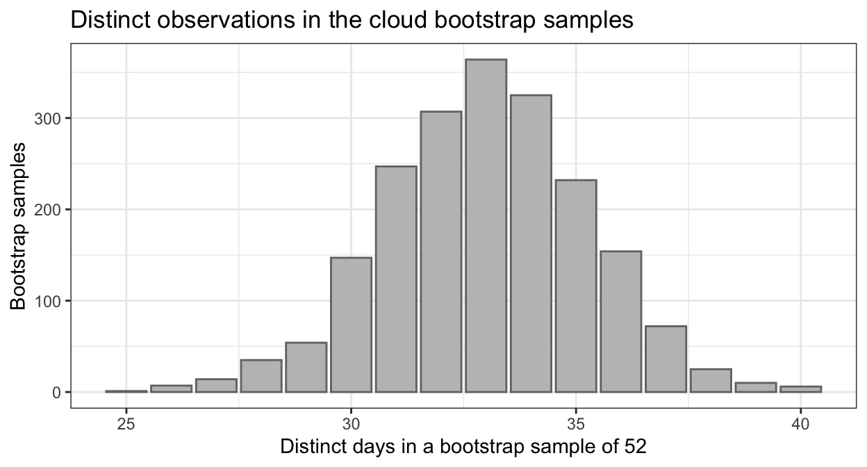

The bootstrap samples contain between 25 and 40 distinct days, 33.0 on average, or 63.5% of the 52.

19.5.1 Inclusion probability

Each of the $n$ draws that make up a bootstrap sample picks observation $j$ with probability $1/n$, independently of the other draws. So

\[P\left(\text{observation } j \text{ not chosen on one draw}\right) = 1 - \frac{1}{n}, \qquad P\left(\text{observation } j \notin Z^{*b}\right) = \left(1 - \frac{1}{n}\right)^n,\]

and the probability that observation $j$ appears in the bootstrap sample is

\[P\left(\text{observation } j \in Z^{*b}\right) = 1 - \left(1 - \frac{1}{n}\right)^n \longrightarrow 1 - e^{-1} \approx 0.632 \quad \text{as } n \to \infty,\]

using $\lim_{n \to \infty} (1 + x/n)^n = e^x$ with $x = -1$. The number of distinct observations in $Z^{*b}$ is $\sum_{j=1}^n \mathrm{I}\left(\text{observation } j \in Z^{*b}\right)$, so by linearity of expectation

\[E\left[\sum_{j=1}^n \mathrm{I}\left(\text{observation } j \in Z^{*b}\right)\right] = n\left[1 - \left(1 - \frac{1}{n}\right)^n\right].\]

For the 52 cloud seeding days, $1 - (1 - 1/52)^{52} = 0.636$, so a bootstrap sample is expected to contain 33.1 distinct days, against the 33.0 averaged over the 2,000 samples above. The figure plots the inclusion probability against $n$, with a dashed line at $1 - e^{-1}$ and a point at $n = 52$.

Code

inclusion_plot <- tibble(n = 1:100) |>
  mutate(p = p_incl(n)) |>
  ggplot(aes(x = n, y = p)) +
  geom_hline(yintercept = 1 - exp(-1), linetype = "dashed") +
  geom_line() +
  geom_point(data = tibble(n = nrow(clouds), p = p_incl(nrow(clouds))),
             size = 3, shape = 21, fill = "white") +
  labs(x = "Sample size n",
       y = "P(observation j in bootstrap sample)",
       title = "Inclusion probability 1 - (1 - 1/n)^n")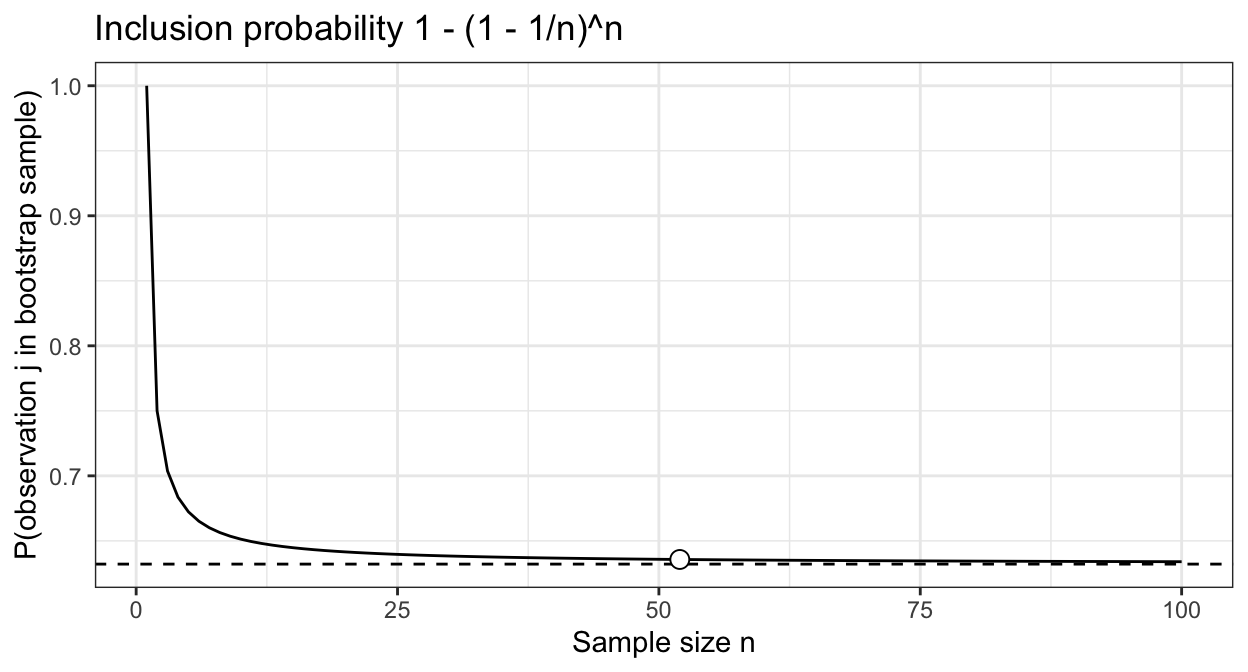

The inclusion probability is 0.75 at $n = 2$ and falls quickly toward $1 - e^{-1} = 0.632$; by $n = 20$ it is 0.642.

19.5.2 Test error

A bootstrap sample could serve as a training set: fit the model to $Z^{*b}$, predict the original $n$ observations, and average the error over $b$. About 63.2% of the observations being predicted were also used to fit the model, some of them several times, so this estimate mixes training error into test error and is too optimistic, increasingly so for flexible models that fit their training data closely. Cross-validation, the subject of the cross-validation lecture, avoids the overlap: each fold’s held-out observations are not in the data the model is fit to.

19.6 Limitations

The bootstrap replaces the population with the sample, so it is only as good as that replacement.

Small samples. A small sample may miss the population’s tails, and the bootstrap cannot reproduce what the sample does not contain. Even for a well-behaved statistic, $\text{SE}_B$ is an estimate with sampling error, as the Accuracy subsection showed at 26 days per treatment, and that error shrinks only as $n$ grows, as the first tab below shows for $\hat\theta$.
Heavy-tailed or skewed populations with a mean-type statistic. A mean of a heavy right tail is driven by its few largest values. The first tab compares $\text{SE}_B$ with the true standard error for $\hat\theta$ and for the ratio of mean rainfall, $\bar y_S/\bar y_U$, where $\bar y_S$ and $\bar y_U$ are the sample mean rainfall on seeded and unseeded days, over simulated experiments of three sizes.
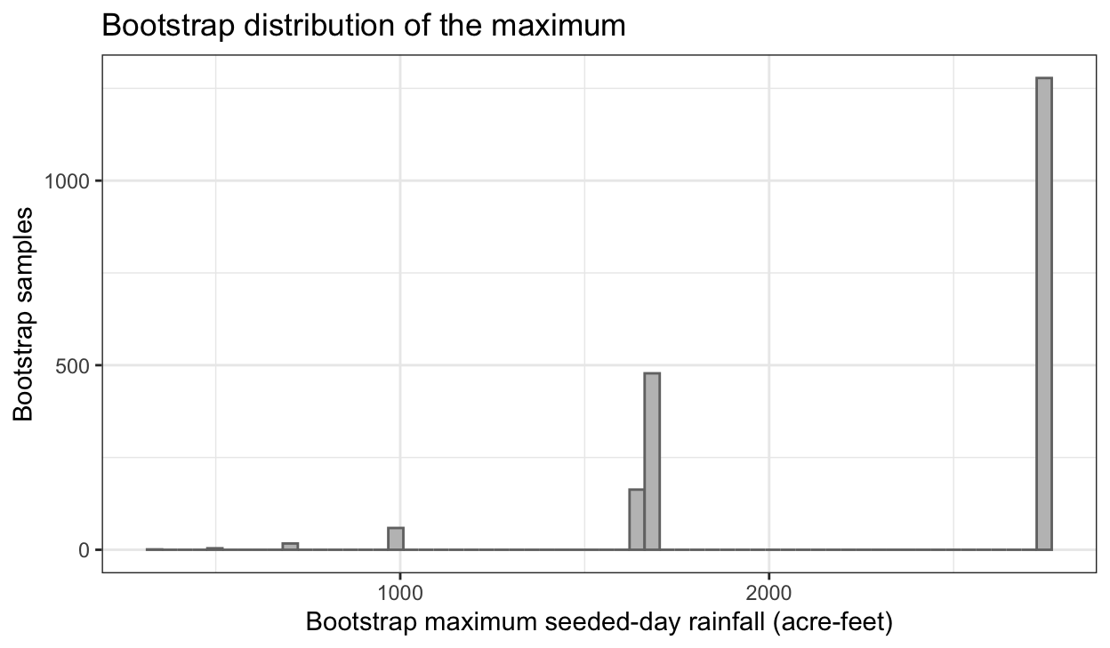
Extreme statistics. The bootstrap maximum can never exceed the sample maximum, and it equals the sample maximum whenever that observation is drawn, with probability $1 - (1 - 1/n)^n$. The second tab shows the bootstrap distribution of the maximum rainfall on a seeded day, from the 2,000 cloud bootstrap samples.
Dependent data. Resampling individual observations assumes they are independent. Temperatures on consecutive days or repeated measurements on the same subject are correlated, and resampling them one at a time breaks that correlation, which usually makes $\text{SE}_B$ too small.

Code

# The ratio of mean rainfall, and its bootstrap SE, on the cloud data.
ratio_of_means <- function(d) {
  mean(d$Rainfall[d$seeded == 1]) / mean(d$Rainfall[d$seeded == 0])
}
ratio_hat <- ratio_of_means(clouds)
boot <- boot |> mutate(ratio = map_dbl(i, \(i) ratio_of_means(clouds[i, ])))
se_boot_ratio <- sd(boot$ratio)

# True SEs and bootstrap SEs at three numbers of days per treatment. The
# 26-day experiments are the ones already bootstrapped in the Accuracy
# subsection; the larger sizes reuse the same functions.
sizes <- c(m_cloud, 100, 400)
size_true <- bind_rows(
  tibble(m = m_cloud, theta = se_true[["theta"]], ratio = se_true[["ratio"]]),
  map(sizes[-1], \(m) {
    st <- simulate_stats(m, n_experiments)
    tibble(m = m, theta = sd(st$theta), ratio = sd(st$ratio),
           ratio_mcse = sd(tapply(st$ratio,
                                  rep(1:20, each = n_experiments / 20),
                                  sd)) / sqrt(20) / sd(st$ratio))
  }) |> list_rbind())
size_checks <- bind_rows(checks,
                         map(sizes[-1], \(m) check_experiments(m, n_check,
                                                               B_check))) |>
  left_join(size_true, by = "m") |>
  transmute(m,
            theta = se_b_theta / theta,
            ratio = se_b_ratio / ratio)
size_summary <- size_checks |>
  pivot_longer(c(theta, ratio), names_to = "stat", values_to = "relative") |>
  group_by(stat, m) |>
  summarize(within = mean(abs(relative - 1) <= 0.25),
            median = median(relative), .groups = "drop")
size_of <- function(st, mm, col) {
  size_summary[[col]][size_summary$stat == st & size_summary$m == mm]
}

limit_labels <- c(theta = "Ratio of geometric means",
                  ratio = "Ratio of means")
size_plot <- size_checks |>
  pivot_longer(c(theta, ratio), names_to = "stat", values_to = "relative") |>
  mutate(stat = factor(limit_labels[stat], levels = limit_labels)) |>
  ggplot(aes(x = factor(m), y = relative)) +
  annotate("rect", xmin = -Inf, xmax = Inf, ymin = 0.75, ymax = 1.25,
           alpha = 0.15) +
  geom_hline(yintercept = 1, linewidth = 0.9) +
  geom_boxplot(outlier.size = 0.8) +
  scale_y_log10() +
  facet_wrap(~ stat) +
  labs(x = "Days per treatment",
       y = "Bootstrap SE divided by true SE (log scale)",
       title = sprintf("%d simulated experiments per size; shaded band: within 25%%",
                       n_check))

seeded_max <- max(clouds$Rainfall[clouds$seeded == 1])
boot <- boot |>
  mutate(max_seeded = map_dbl(i, \(i) {
    max(clouds$Rainfall[i][clouds$seeded[i] == 1])
  }))
share_at_max <- mean(boot$max_seeded == seeded_max)
max_plot <- ggplot(boot, aes(x = max_seeded)) +
  geom_histogram(bins = 60, fill = "grey75", color = "grey45") +
  labs(x = "Bootstrap maximum seeded-day rainfall (acre-feet)",
       y = "Bootstrap samples",
       title = "Bootstrap distribution of the maximum")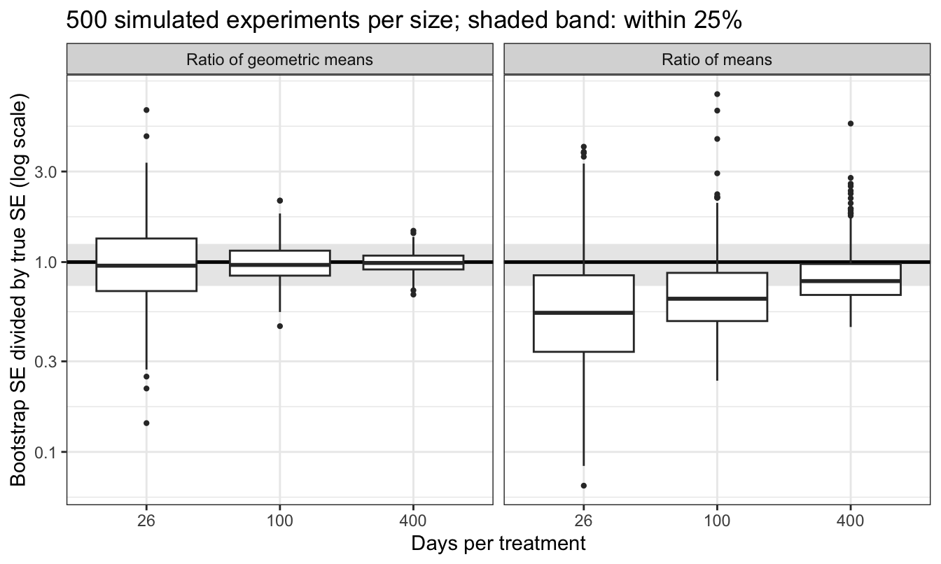

Under the known population, log rainfall is normal with a common $\sigma$ in both treatments, so the mean rainfall on a day with seeding indicator $D$ is $e^{\beta_0 + \beta_1 D + \sigma^2/2}$, and the ratio of means $\mu_S/\mu_U$ also equals $\theta$, where $\mu_S$ and $\mu_U$ are the population mean rainfall on seeded and unseeded days. The two statistics estimate the same quantity, but at 26 days per treatment the ratio of means $\bar y_S/\bar y_U$ has true standard error 3.66 (accurate to about $$4%), against 1.65 for $\hat\theta$.

The table gives, for each statistic and size, the percentage of the 500 simulated experiments whose $\text{SE}_B$ fell within 25% of the true standard error. With 500 experiments each percentage is accurate to about $$4 percentage points or better (two binomial standard errors).

Statistic	26 days per treatment	100 days per treatment	400 days per treatment
Ratio of means	17%	30%	49%
Ratio of geometric means	41%	73%	97%

For the ratio of geometric means the percentage climbs quickly with $n$, as its $\text{SE}_B$ inherits the shrinking error of $\hat\theta$. For the ratio of means it is lower at every size and reaches only 49% at 400 days per treatment. The median ratio of $\text{SE}_B$ to the truth for the ratio of means is 0.54, 0.64, and 0.79 at the three sizes (each true standard error is from 100,000 experiments, accurate to about $$4% or better), so its $\text{SE}_B$ is typically too small.

A likely reason is that a sample seldom holds the population’s rare, very wet days in their population proportion: it usually holds too few, giving an $\text{SE}_B$ that is too small, and occasionally holds several, giving one far too large, and the bootstrap resamples only the days the sample contains. On the log scale those days are not extreme. The two bootstrap standard errors therefore err for different reasons: that of the ratio of geometric means is noisy because $\text{SE}(\hat\theta)$ is proportional to $\theta$, which is known only through $\hat\theta$, while that of the ratio of means is also biased low by the heavy right tail. On the cloud data the ratio of means is 2.69 with $\text{SE}_B = 1.51$, likely well below its true standard error.

In the cloud bootstrap samples, 63.9% of the bootstrap maxima equal the sample maximum of 2,745.6 acre-feet, against $1 - (1 - 1/52)^{52} = 63.6$% expected. Most of the bootstrap distribution is a single spike at the sample maximum, so it carries no information about how far the population maximum lies above the sample’s.

Beyond this course

The delta method gives an approximate formula standard error for a smooth function of estimates from a first-order Taylor expansion; for $\hat\theta = e^{\hat\beta_1}$ it is $\hat\theta\,\text{SE}(\hat\beta_1)$.
Out-of-bag error repairs the bootstrap’s test-error estimate by predicting each observation only from bootstrap samples that left it out; it reappears with bagging and random forests (ISLR2 Chapter 8).
The parametric bootstrap resamples from a fitted model rather than from the data, much as the known-population simulation above drew experiments from the fitted log-scale regression.
Bias-corrected and accelerated (BCa) and bootstrap-$t$ intervals improve on the percentile interval’s coverage in small or skewed samples.
The block bootstrap resamples blocks of consecutive observations to keep the dependence in a time series, and stratified resampling draws within each group (here, 26 days from each treatment) to match a design with fixed group sizes.

19.7 Conclusion

The standard error of a statistic is the standard deviation of its sampling distribution. Simple formulas give it for a few statistics, such as a mean or a regression coefficient, and lm() reports it for each coefficient but not for a function of the coefficients, such as an exponentiated coefficient. A median, a quantile, an AUC, and many statistics computed by an algorithm have no simple formula. The bootstrap estimates the standard error by treating the sample as the population: draw $B$ bootstrap samples of $n$ observations with replacement, compute the statistic on each, and take the standard deviation of the $B$ results. Where a formula exists, such as for a regression coefficient, the two estimate the same standard error and can be checked against each other; where no simple formula is available, the bootstrap is computed in exactly the same way. A bootstrap standard error is itself an estimate, and for a statistic whose standard error grows with the parameter, such as a ratio, it is no more accurate than the estimate itself.

The bootstrap distribution gives two confidence intervals. The percentile interval takes the $\alpha/2$ and $1 - \alpha/2$ quantiles of the bootstrap statistics, follows any skew, and moves with a monotone transformation of the statistic; the normal-approximation interval is $\hat\theta \pm z_{1-\alpha/2}\,\text{SE}_B(\hat\theta)$ and is symmetric. They agree when the bootstrap distribution is approximately normal and centered at $\hat\theta$, and skewness or bias separates them.

A bootstrap sample contains each observation with probability $1 - (1 - 1/n)^n$, which approaches $1 - 1/e \approx 0.632$, so a model fit to a bootstrap sample and evaluated on the original data is evaluated mostly on its own training observations; cross-validation, not the bootstrap, estimates test error. Bootstrap standard errors and intervals are unreliable for small samples, for heavy-tailed or skewed populations summarized by a mean-type statistic, for extreme statistics such as the maximum, and for dependent data resampled one observation at a time.

The next lecture begins regularization (ISLR2 Sections 6.1-6.2): selecting a subset of the features, and shrinking the least squares coefficient estimates toward zero with ridge regression and the lasso, with cross-validation choosing how much.