explain how a support vector classifier fit to polynomial features of the explanatory variables gives a curved boundary in the explanatory variables, and compute how fast the number of such features grows with the number of explanatory variables and the degree,
state that the support vector classifier classifies a new observation through its inner products with the support vectors alone, \(\hat f(x) = \hat w_0 + \sum_{i \in \mathcal{S}}\hat\alpha_i
\langle x, x_i\rangle\), define the support vector machine as that classifier with the inner product replaced by a kernel \(K(x, x_i)\), and write the linear, polynomial, and radial kernels,
derive that the polynomial kernel of degree 2 is the inner product of an enlarged set of features, and explain why the radial kernel is local and how its \(\gamma\) trades bias against variance,
choosecost and \(\gamma\) by 10-fold cross-validation over a two-dimensional grid with e1071::tune(), and evaluate the chosen support vector machine against the linear support vector classifier by test error rate and confusion matrix,
describe the one-versus-one and one-versus-all approaches to more than two classes, and explain how svm() classifies by one-versus-one voting,
derive the hinge-loss-plus-penalty form of the support vector classifier, and compare the hinge loss with the logistic regression loss, including what each classifier outputs.
This is the last of three lectures on support vector machines. The previous two fit a flat boundary, a hyperplane, with a margin that the support vector classifier lets observations violate at a price cost. This lecture curves the boundary. The reading is ISLR2 Sections 9.3 to 9.5.
32.1 Sacramento homes
Question. Within the Sacramento metropolitan area, can a home’s location alone tell whether it is in the city of Sacramento or in one of the cities around it?
Data.modeldata::Sacramento records 932 home sales reported in the Sacramento area over five days in May 2008, with each home’s city and its location as longitude and latitude in degrees. The observations are homes. The class is the city, coded \(y_i = 1\) for Sacramento, the second level of the factor, and \(y_i = -1\) for Other, any of the 36 other cities. The two explanatory variables are longitude and latitude.
# Homes, with the class coded y = 1 (Sacramento) or y = -1 (Other).homes <- modeldata::Sacramento |>mutate(place =if_else(city =="SACRAMENTO", "Sacramento", "Other"),place =factor(place, levels =c("Other", "Sacramento")),y =if_else(place =="Sacramento", 1, -1))count(homes, place)
# A tibble: 2 x 2
  place          n
  <fct>      <int>
1 Other        494
2 Sacramento   438
Two thirds of the homes, chosen at random, are the training homes; the rest are the test homes, used only to evaluate the chosen classifiers.
# Two thirds of the homes for training, the rest for testing.n_train <-round(2*nrow(homes) /3)train_rows <-sample(nrow(homes), n_train)train <- homes[train_rows, ]test <- homes[-train_rows, ]count(train, place)
# A tibble: 2 x 2
  place          n
  <fct>      <int>
1 Other        327
2 Sacramento   294
NoteCode
# Standard deviations of the two coordinates among the training homes.s_train <-sapply(train[c("longitude", "latitude")], sd)# Axes in degrees every 0.2, minor lines midway; longitude labeled in# degrees west.x_scale <-scale_x_continuous(breaks =seq(-121.6, -120.6, by =0.2),minor_breaks =seq(-121.5, -120.7, by =0.2),labels =function(x) {format(abs(x), nsmall =1) })y_scale <-scale_y_continuous(breaks =seq(38.2, 39, by =0.2),minor_breaks =seq(38.3, 38.9, by =0.2),labels =function(x) {format(x, nsmall =1) })x_limits <-c(-121.62, -120.55)y_limits <-c(38.18, 39.05)stopifnot(between(range(homes$longitude), x_limits[1], x_limits[2]),between(range(homes$latitude), y_limits[1], y_limits[2]))# The homes' axes: one standard deviation of each coordinate the same# length; the legend in the empty lower-right corner.home_base <-function() {ggplot(mapping =aes(x = longitude, y = latitude)) + x_scale + y_scale +coord_fixed(ratio = s_train[["longitude"]] / s_train[["latitude"]],xlim = x_limits, ylim = y_limits, expand =FALSE) +scale_color_manual(values = place_colors) +scale_shape_manual(values = place_shapes) +labs(x ="Longitude (degrees west)", y ="Latitude (degrees north)",color ="City", shape ="City") +theme(legend.position ="inside",legend.position.inside =c(0.97, 0.03),legend.justification =c(1, 0))}# The points on top of any regions or lines drawn before them.home_points <-function(data = train, class ="place") {geom_point(data = data,aes(color = .data[[class]], shape = .data[[class]]),size =1.6)}home_plot <-home_base() +home_points()# Kilometers per degree of latitude, and per degree of longitude here.km_lat <-111.2km_lon <- km_lat *cos(mean(train$latitude) * pi /180)
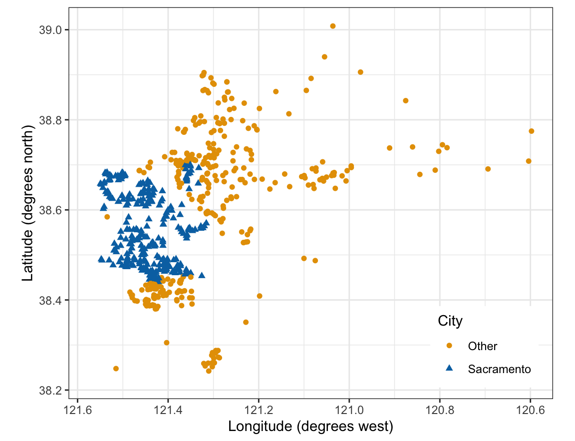
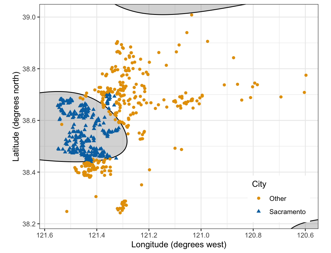
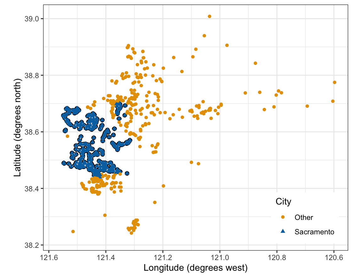
The training homes in the city of Sacramento form a block in the west of the area. Homes in other cities lie north, east, and south of that block, and a few lie west of it. No straight line puts the Sacramento homes on one side and the others on the other: any line through the block leaves other cities on both sides. The axes are drawn so that one standard deviation of each coordinate among the training homes, \(s_{\texttt{longitude}} = 0.1367\) and \(s_{\texttt{latitude}} = 0.1375\) degrees, has the same length, since svm() standardizes both. A degree of longitude here is about 87 km and a degree of latitude about 111 km, so the figure is wider than a map.
32.2 Enlarged feature space
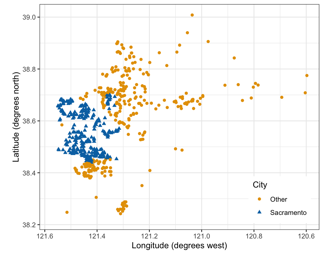
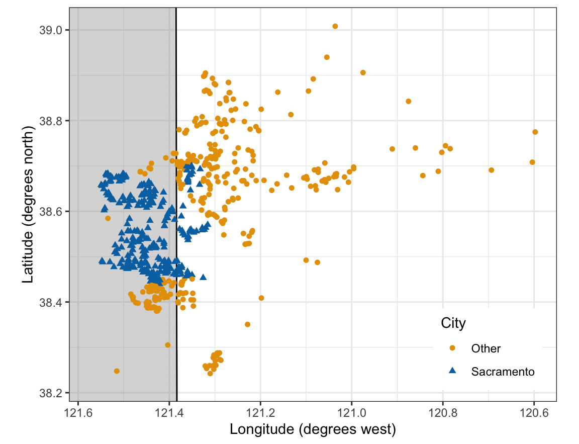
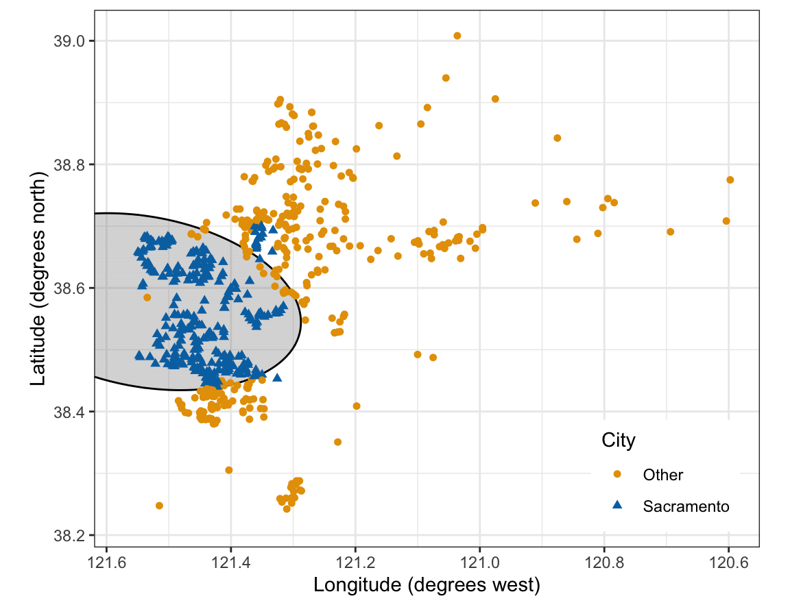
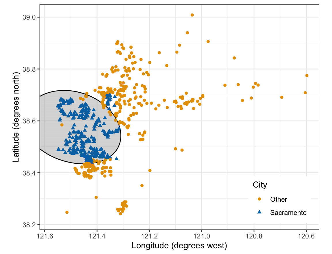
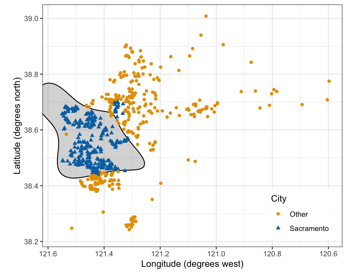
The tabs show the training homes, and then three support vector classifiers, each the linear-kernel svm() of the previous lecture fit to all the polynomial features of the two coordinates up to degree \(d\), for \(d = 1\) (the coordinates themselves), 2, and 3. Each shades the region classified Sacramento and draws the boundary \(\hat f(x) = 0\).
NoteCode
# Standardized coordinates z1 and z2, with the training means and standard# deviations, so that powers and products stay on a common scale.center_train <-colMeans(train[c("longitude", "latitude")])add_z <-function(data) {mutate(data,z1 = (longitude - center_train[["longitude"]]) / s_train[["longitude"]],z2 = (latitude - center_train[["latitude"]]) / s_train[["latitude"]])}train <-add_z(train)test <-add_z(test)# A grid covering the plot, for drawing a fit's regions.grid_x <-seq(x_limits[1], x_limits[2], length.out =250)grid_y <-seq(y_limits[1], y_limits[2], length.out =250)grid <-expand_grid(longitude = grid_x, latitude = grid_y) |>add_z()# svm()'s decision values with Sacramento positive. Their sign is set by# the class of the first training observation, which the column name# shows first.decision_of <-function(fit, data) { pred <-predict(fit, data, decision.values =TRUE) decision <-attr(pred, "decision.values") flip <-if (colnames(decision) =="Sacramento/Other") 1else-1stopifnot(colnames(decision) %in%c("Sacramento/Other","Other/Sacramento")) flip *drop(decision)}# A fit's Sacramento region shaded, its boundary drawn, homes on top.region_plot <-function(fit, data = train) { grid_fit <-mutate(grid, f_hat =decision_of(fit, grid))home_base() +geom_tile(data =filter(grid_fit, f_hat >0),width =diff(grid_x)[1], height =diff(grid_y)[1],fill ="grey55", alpha =0.35) +geom_contour(data = grid_fit, aes(z = f_hat),breaks =0, color ="black") +home_points(data)}# Support vector classifiers on polynomial features of degree 1, 2, 3.degrees <-1:3poly_fits <-lapply(degrees, function(d) { model <-as.formula(paste0("place ~ poly(z1, z2, degree = ", d,", raw = TRUE)"))svm(model, data = train, kernel ="linear", cost =1)})poly_plots <-lapply(poly_fits, region_plot)# Training error rates and feature counts of the three fits.error_of <-function(fit, data, class ="place") {mean(predict(fit, data) != data[[class]])}poly_errors <-sapply(poly_fits, error_of, data = train)n_features <-choose(2+ degrees, degrees) -1stopifnot(poly_fits[[2]]$tot.nSV < poly_fits[[1]]$tot.nSV)
The support vector classifier draws a hyperplane in whatever features it is given. Given the \(p = 2\) explanatory variables, the standardized longitude and latitude \(X_1\) and \(X_2\), alone, it draws a line (degree 1). Given the degree-2 features \(X_1, X_2, X_1^2, X_1X_2, X_2^2\), it draws a hyperplane
in five dimensions, where the \(\hat w_j\) are the rescaled estimates of the previous lecture’s penalty form, one per feature. In general, all the monomials of degree at most \(d\) in \(p\) explanatory variables, without the constant, are
\[
q = \binom{p + d}{d} - 1
\]
features, \(q = 5\) here. poly() with raw = TRUE builds them from the standardized coordinates z1 and z2, and svm() with a linear kernel fits the hyperplane; svm() standardizes each of the five features again, so the \(\hat w_j\) are per standard deviation of each feature:
# Support vector classifier on the degree-2 features of z1 and z2.svc_quad <-svm(place ~poly(z1, z2, degree =2, raw =TRUE),data = train, kernel ="linear", cost =1)# Training error rate.mean(predict(svc_quad, train) != train$place)
[1] 0.06602254
Read as an equation in \(X_1\) and \(X_2\), the hyperplane is a conic section: an ellipse, a parabola, or a hyperbola. The degree-2 fit’s boundary is an ellipse around the city’s block. Degree 3 adds the four cubic features, and the boundary becomes a cubic curve, which also gives Sacramento two regions at the edge of the plot, far from any home. This is the feature engineering of the regression lectures, with a hyperplane in place of least squares. The training error rates of the three fits, all with cost = 1, are 20.1%, 6.6%, and 6.3%.
32.2.2 Feature count
The number of features \(q = \binom{p + d}{d} - 1\) is 5 for \(p = 2\) and \(d = 2\) and 9 for \(d = 3\). It grows fast with \(p\): with \(p = 10\) explanatory variables, degree 3 already gives \(q = 285\) features and degree 5 gives \(q = 3{,}002\). Each must be computed for every observation and enter every inner product the solver computes, and the boundary is still limited to polynomials of the chosen degree.
32.3 Kernels
The data are the training homes of the first figure. The question is how to get a curved boundary like those in the tabs above without listing the enlarged features.
32.3.1 Inner products
Write \(\langle x_i, x_{i'}\rangle = \sum_{j=1}^p x_{ij}x_{i'j}\) for the inner product of two observations, with \(x_i\) the \(p\) standardized explanatory variables that svm() uses. (On enlarged features the sum runs over the \(q\) features instead; here and in the kernels below it runs over the \(p\) explanatory variables.) The support vector classifier’s fitted normal vector is a weighted sum of the support vectors, \(\hat w = \sum_{i \in \mathcal{S}}\hat\alpha_i x_i\) (the form svm() stores, coefs times SV, in the previous lectures). Therefore a new observation \(x\) is classified by
\(\hat\alpha_i\) is the weight of support vector \(i\), positive for \(y_i = 1\) and negative for \(y_i = -1\) (svm()’s coefs, in its sign), zero for every other observation, and
\(\hat w_0\) is the rescaled intercept (ISLR2 writes \(\beta_0\), which here is the unit-norm intercept).
So classifying a new observation needs only its inner products with the support vectors. (The weights can also be computed from the inner products of the training observations alone; that is not derived here, see the callout at the end.)
32.3.2 Kernel functions
A kernel\(K(x_i, x_{i'})\) is a function of two observations that replaces the inner product. The support vector machine is the support vector classifier with a kernel,
is the vector of degree-2 features of observation \(i\), up to constant multiples; its constant 1 adds the same amount to every inner product, and is absorbed by \(\hat w_0\). A support vector machine with this kernel is the support vector classifier on those features, with a boundary that is a conic section. Computing the kernel takes one inner product over the \(p\) explanatory variables and one power, whatever the number of features \(q = \binom{p+d}{d} - 1\).
32.3.4 Radial kernel
The radial kernel is 1 when \(x = x_i\) and falls toward 0 as \(x\) moves away from \(x_i\). In \(\hat f\left(x^*\right) = \hat w_0 + \sum_{i \in
\mathcal{S}}\hat\alpha_i K\left(x^*, x_i\right)\), a support vector far from a new observation \(x^*\) contributes almost nothing, so \(x^*\) is classified by the support vectors near it: the radial kernel is local. \(\gamma\) sets how near. \(K\) falls to 0.01 at distance \(\sqrt{\log(100)/\gamma}\) standard deviations, so a large \(\gamma\) makes each support vector’s influence small in extent and a small \(\gamma\) makes it wide. The radial kernel is also an inner product of enlarged features, but of infinitely many, so no explicit enlargement could reproduce it.
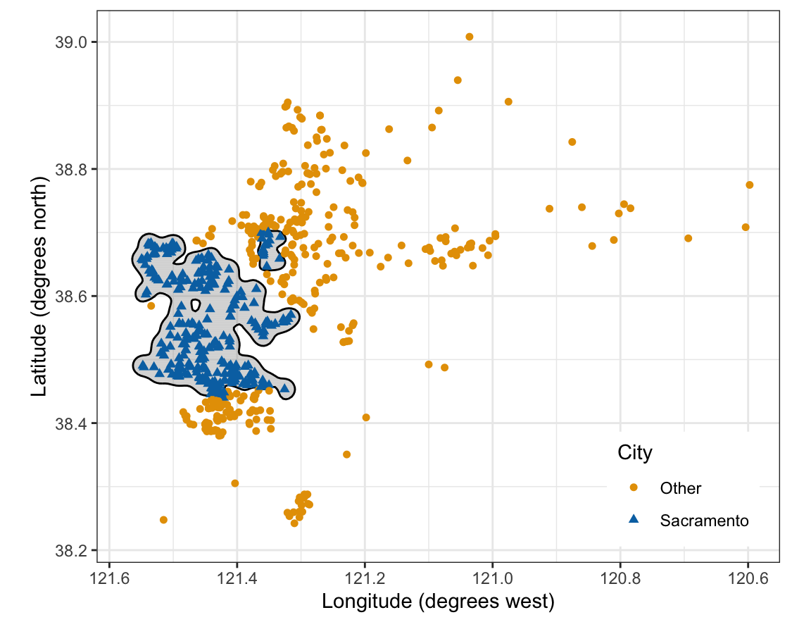
The tabs show four support vector machines with the radial kernel, fit with svm(kernel = "radial") (the Fitting subsection below shows the call), all with the cost that cross-validation chooses below, at four values of \(\gamma\).
NoteCode
# Radial-kernel fits with cost = 10 at four values of gamma.tab_cost <-10tab_gammas <-c(0.1, 1, 100, 1000)gamma_fits <-lapply(tab_gammas, function(g) {svm(place ~ longitude + latitude, data = train, kernel ="radial",cost = tab_cost, gamma = g)})gamma_plots <-lapply(gamma_fits, region_plot)# Training error rates and support vector counts of the four fits.gamma_errors <-sapply(gamma_fits, error_of, data = train)gamma_nsv <-sapply(gamma_fits, function(fit) { fit$tot.nSV})stopifnot(!is.unsorted(rev(gamma_errors)))# Far from every support vector the largest-gamma fit is w0, which puts# such a home in Other: -rho in svm()'s sign, Sacramento positive.stopifnot(train$place[1] =="Sacramento", gamma_fits[[4]]$rho >0)
At \(\gamma\) = 0.1 each support vector’s influence reaches 6.8 standard deviations, about the width of the whole area, and the boundary is a smooth oval: low variance, more bias. As \(\gamma\) grows, the boundary follows the city’s block more closely, and the training error rate falls from 6.3% to 0.0%. At \(\gamma\) = 1000 the influence reaches only 0.07 standard deviations: the region classified Sacramento breaks into small islands around the training homes, 581 of the 621 training homes are support vectors, and a new home between the islands is too far from every support vector for any to count, so \(\hat f\) there is \(\hat w_0\) and the home gets the class its sign gives, Other. That is low bias and high variance. \(\gamma\) = 100 with cost = 10, the pair cross-validation chooses below, already has training error rate 0.0% with 350 support vectors: it sits at the edge of that overfitting regime.
32.3.5 Fitting
svm() with kernel = "radial" fits the support vector machine with the radial kernel; gamma is \(\gamma\) (in e1071, as in libsvm). As in the previous lecture, svm() standardizes the features by default, so the kernel’s distances are in standard deviations.
Call:
svm(formula = place ~ longitude + latitude, data = train, kernel = "radial",
    cost = 1, gamma = 1)


Parameters:
   SVM-Type:  C-classification
 SVM-Kernel:  radial
       cost:  1

Number of Support Vectors:  147
NoteCode
# The kernel form by hand: svm()'s decision value is# sum over support vectors of coefs times K(x, x_i), minus rho.z_test <-scale(as.matrix(test[c("longitude", "latitude")]),center = svm_fit$x.scale[["scaled:center"]],scale = svm_fit$x.scale[["scaled:scale"]])squared_distance <-outer(rowSums(z_test^2), rowSums(svm_fit$SV^2), "+") -2* z_test %*%t(svm_fit$SV)kernel_matrix <-exp(-svm_fit$gamma * squared_distance)by_hand <-drop(kernel_matrix %*% svm_fit$coefs) - svm_fit$rhopred_test <-predict(svm_fit, test, decision.values =TRUE)stopifnot(isTRUE(all.equal(by_hand,drop(attr(pred_test, "decision.values")),check.attributes =FALSE)))# The first training home is in Sacramento, so svm()'s decision values# are positive for Sacramento.stopifnot(train$place[1] =="Sacramento",colnames(attr(pred_test, "decision.values")) =="Sacramento/Other")
The fitted object holds the support vectors SV (standardized), their weights \(\hat\alpha_i\) as coefs, and \(-\hat w_0\) as rho, in svm()’s sign, positive here for Sacramento, the class of the first training home. Summing coefs times the radial kernel over the 147 support vectors, minus rho, reproduces svm()’s decision values for the test homes.
32.4 Tuning
32.4.1 Grid
The radial kernel has two tuning parameters, cost and \(\gamma\), chosen together by 10-fold cross-validation over a grid of pairs. The estimate for each pair is \(\text{CV}_{(10)}(\texttt{cost}, \gamma)\), the equal-weight mean of the fold error rates as in the previous lecture. tune() takes a list of values for each, and fits every pair.
# 10-fold cross-validation over a grid of cost and gamma.cv_svm <-tune(svm, place ~ longitude + latitude, data = train,kernel ="radial",ranges =list(cost =10^(-1:3), gamma =10^(-2:3)))cv_svm$best.parameters
   cost gamma
23   10   100
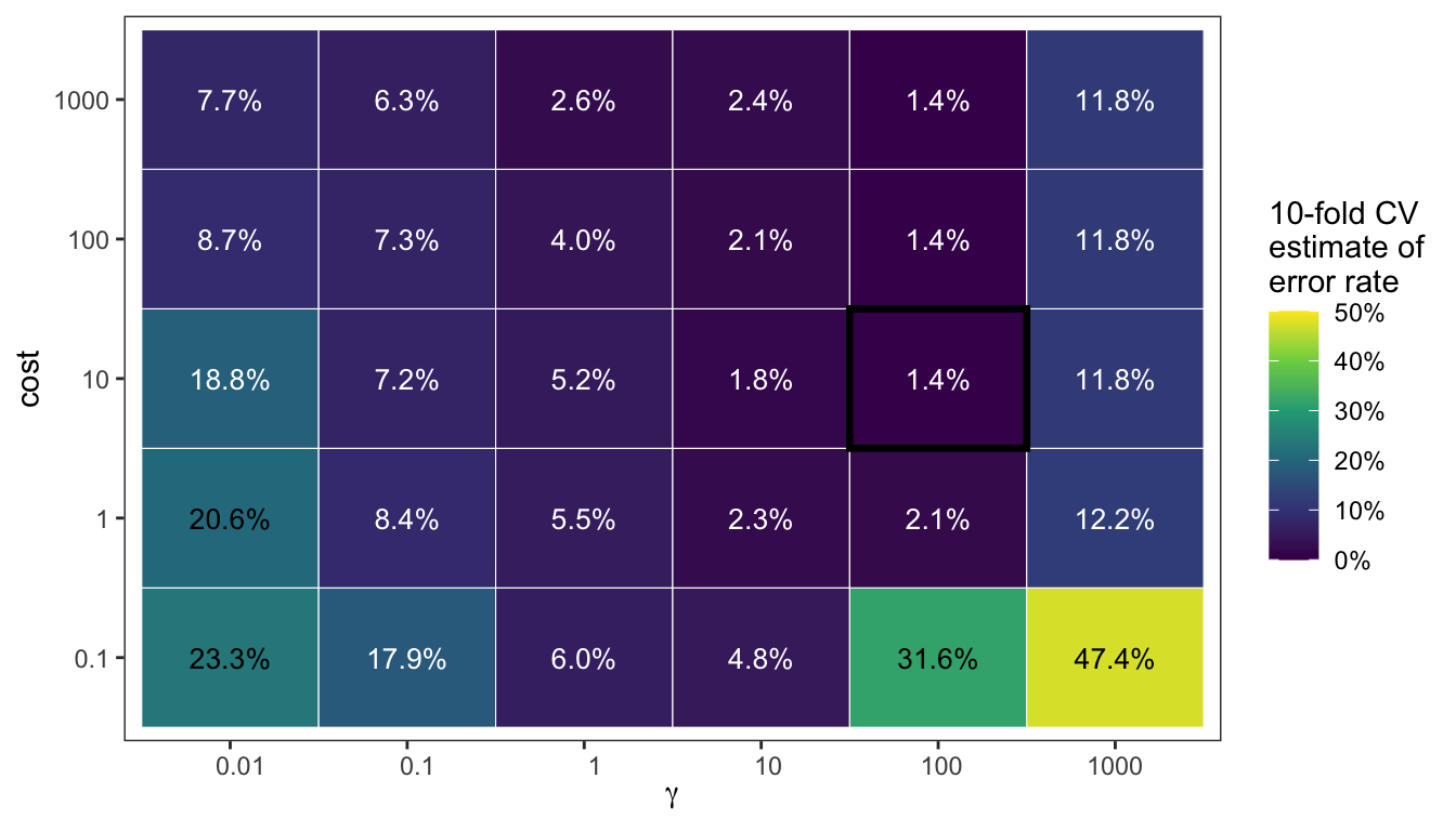
The figure shows \(\text{CV}_{(10)}(\texttt{cost}, \gamma)\) for each pair, with the chosen pair outlined.
NoteCode
# The cross-validation estimate for each pair, and the chosen pair.cv_table <-as_tibble(cv_svm$performances)best <- cv_svm$best.parametersbest_row <-filter(cv_table, cost == best$cost, gamma == best$gamma)# The gamma tabs above use the chosen cost and show the chosen gamma.stopifnot(tab_cost == best$cost, tab_gammas[3] == best$gamma)# Discrete axes, labeled as the values themselves.cv_cells <- cv_table |>mutate(cost_label =factor(format(cost, scientific =FALSE,drop0trailing =TRUE),levels =format(sort(unique(cost)),scientific =FALSE,drop0trailing =TRUE)),gamma_label =factor(format(gamma, scientific =FALSE,drop0trailing =TRUE),levels =format(sort(unique(gamma)),scientific =FALSE,drop0trailing =TRUE)),chosen = cost == best$cost & gamma == best$gamma,label =paste0(fmt(100* error, 1), "%"),text_color =if_else(error >0.2, "black", "white"))cv_plot <-ggplot(cv_cells, aes(x = gamma_label, y = cost_label)) +geom_tile(aes(fill = error), color ="white") +geom_tile(data =filter(cv_cells, chosen),fill =NA, color ="black", linewidth =1.2) +geom_text(aes(label = label, color = text_color), size =3.5) +scale_color_identity() +scale_fill_viridis_c(labels = scales::label_percent(),limits =c(0, 0.5)) +labs(x =expression(gamma), y ="cost",fill ="10-fold CV\nestimate of\nerror rate") +theme(panel.grid =element_blank())# Error rate of classifying every training home Other, the more common.all_other_error <-mean(train$place !="Other")# The estimate at the smallest cost and gamma, and at the largest gamma.corner_small <-filter(cv_table, cost ==min(cost), gamma ==min(gamma))corner_large <-filter(cv_table, cost ==min(cost), gamma ==max(gamma))largest_gamma <-filter(cv_table, gamma ==max(gamma))stopifnot(min(largest_gamma$error) >2* best_row$error)# A linear support vector classifier, tuned over cost as in the previous# lecture.cv_svc <-tune(svm, place ~ longitude + latitude, data = train,kernel ="linear",ranges =list(cost =10^seq(-2, 2, by =0.5)))svc_best <- cv_svc$best.modelsvc_cv_error <-min(cv_svc$performances$error)# Costs whose estimate ties the smallest (to floating-point accuracy).svc_tied <- cv_svc$performances$cost[abs(cv_svc$performances$error - svc_cv_error) <1e-12]stopifnot(abs(corner_large$error - all_other_error) <0.01,abs(corner_small$error - svc_cv_error) <0.05)# Pairs whose estimate ties the smallest.n_tied <-sum(cv_table$error == best_row$error)tied <-filter(cv_table, error == best_row$error)stopifnot(all(tied$gamma == best$gamma), best$cost ==min(tied$cost))tie_note <-if (n_tied >1) {paste0(" (", n_tied, " pairs share it, and `tune()` takes the first,"," the smallest `cost` among them)")} else {""}# The estimate at the smallest and the largest cost, for each gamma: the# largest cost has the smaller estimate at every gamma.by_gamma <- cv_table |>group_by(gamma) |>summarize(small = error[cost ==min(cost)],large = error[cost ==max(cost)])stopifnot(all(by_gamma$large < by_gamma$small))cost_at <-function(g, which) { by_gamma[[which]][by_gamma$gamma == g]}
The smallest estimate, 1.4%, is at cost = 10 and \(\gamma\) = 100 (3 pairs share it, and tune() takes the first, the smallest cost among them). The corners show the two ways to go wrong:
Small \(\gamma\) (left): each support vector’s influence is wide and the boundary nearly linear, too rigid for the city’s block. At the smallest cost and \(\gamma\) the estimate is 23.3%, within a few percentage points of the linear support vector classifier’s smallest estimate, 20.3%.
Large \(\gamma\) (right): each training home makes its own island, the fit overfits, and the estimate rises to at least 11.8% at \(\gamma\) = 1000, whatever cost. With the smallest cost as well, the estimate, 47.4%, is close to the error rate of classifying every home Other, 47.3%.
At every \(\gamma\), cost = 1000 has a smaller estimate than cost = 0.1: a larger cost lets the fit bend further at the price of a narrower margin. The gain is largest where cost = 0.1 fails badly: the estimate falls from 31.6% to 1.4% at \(\gamma\) = 100 and from 47.4% to 11.8% at \(\gamma\) = 1000, against 23.3% to 7.7% at \(\gamma\) = 0.01. The fold error rates at the chosen pair have standard deviation 1.6%, so neighboring cells within a percentage point or so of the smallest are not distinguishable.
32.4.2 Test error
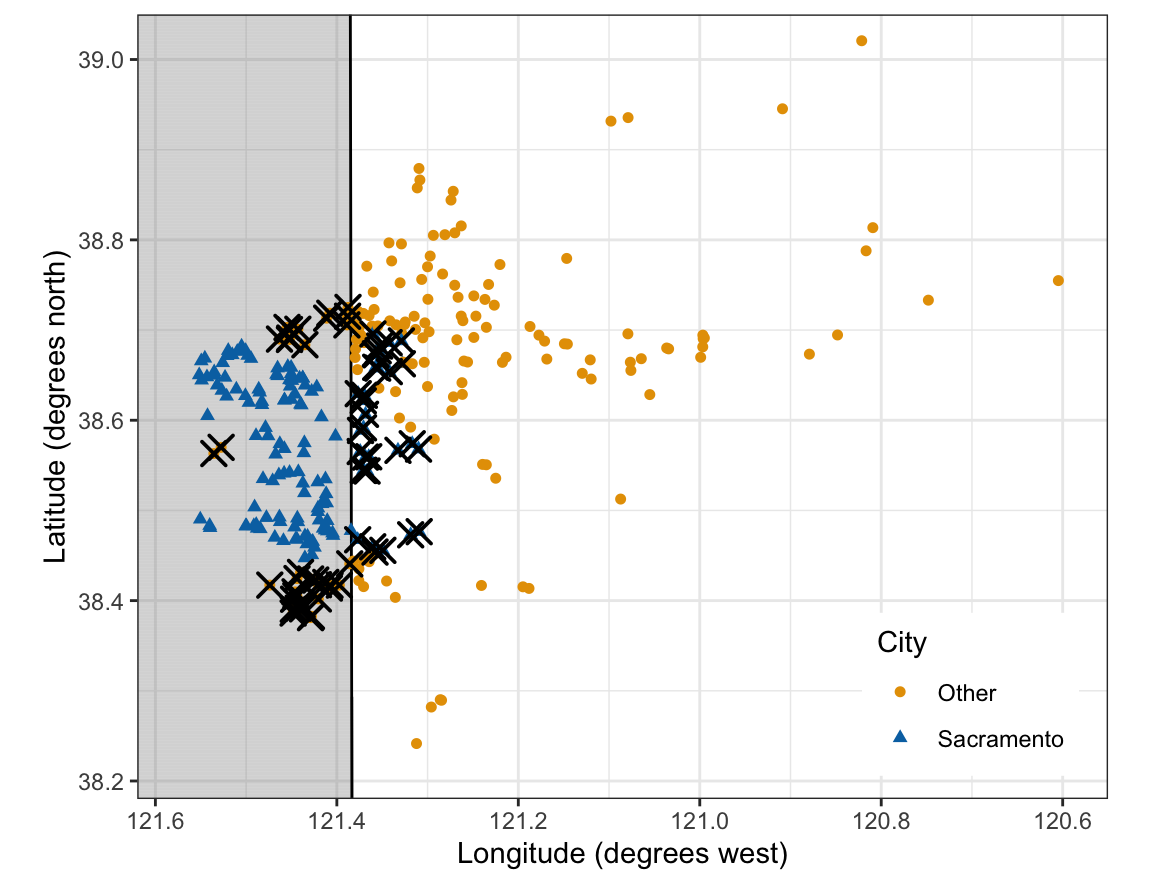
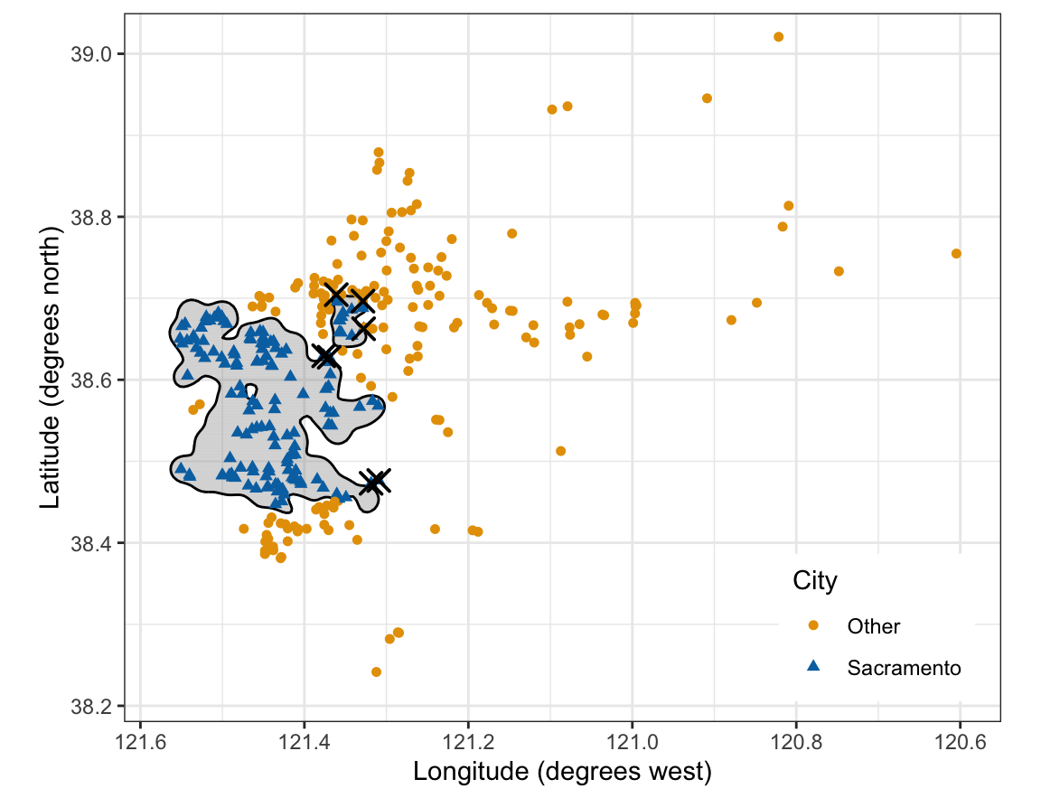
The linear support vector classifier is tuned as in the previous lecture, with tune() over cost from 0.01 to 100, two values per factor of 10. Its estimate, 20.3%, ties at every cost from 0.32 to 100, up to floating-point rounding, and tune() reports the first exact minimum, cost = 1. The tabs show the test homes with the boundaries of that linear support vector classifier and of the support vector machine chosen above, each refit to all the training homes; crosses mark the test homes each misclassifies.
NoteCode
svm_best <- cv_svm$best.model# A fit's regions and boundary over the test homes, misclassified ones# crossed.test_plot <-function(fit) { wrong <-filter(test, predict(fit, test) != place)region_plot(fit, data = test) +geom_point(data = wrong, shape =4, size =3.5, stroke =1)}test_svc_plot <-test_plot(svc_best)test_svm_plot <-test_plot(svm_best)# Test error rates of the linear fit and the radial fit, and of# classifying every test home Other.test_errors <-c(linear =error_of(svc_best, test),radial =error_of(svm_best, test))test_all_other <-mean(test$place !="Other")stopifnot(test_errors[["radial"]] < test_errors[["linear"]] /4)
With Sacramento as the positive class, the confusion matrices of the test homes are
# Truth in the rows, predictions in the columns.list(radial =table(Truth = test$place,Predicted =predict(svm_best, test)),linear =table(Truth = test$place,Predicted =predict(svc_best, test)))
$radial
            Predicted
Truth        Other Sacramento
  Other        165          2
  Sacramento     5        139

$linear
            Predicted
Truth        Other Sacramento
  Other        129         38
  Sacramento    32        112
The support vector machine misclassifies 2.3% of the 311 test homes and the linear support vector classifier 22.5%, against 46.3% for classifying every test home Other. The linear boundary is nearly a north-south line: it misclassifies the homes of other cities west of it, north and south of the city’s block, and the Sacramento homes east of it. The radial boundary encloses the block, and its few errors lie at the city’s edge.
32.5 More than two classes
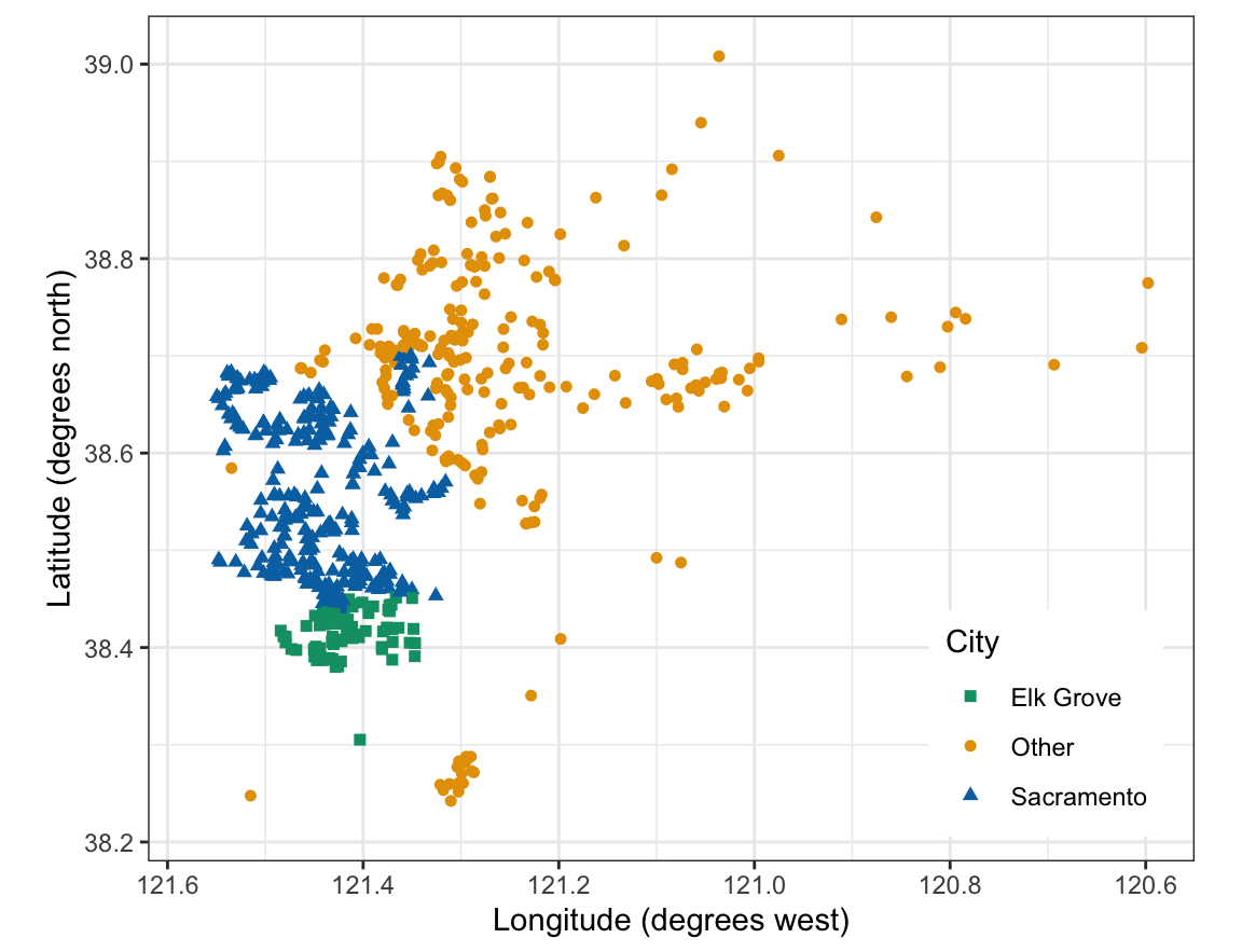
The figure shows the training homes in three classes: the city of Sacramento, the city of Elk Grove, and every other city.
NoteCode
# Three classes: Sacramento, Elk Grove, and every other city.three_levels <-c("Elk Grove", "Other", "Sacramento")add_three <-function(data) { three <-case_when(data$city =="SACRAMENTO"~"Sacramento", data$city =="ELK_GROVE"~"Elk Grove",TRUE~"Other")mutate(data, three =factor(three, levels = three_levels))}train <-add_three(train)test <-add_three(test)three_plot <-home_base() +home_points(class ="three")
All three classes appear: Elk Grove’s homes (squares) form a cluster south of Sacramento’s (triangles), inside the region the two-class fits gave to Other (circles).
32.5.1 One versus one and one versus all
With \(K\) classes, \(K > 2\) (\(K\) without arguments is the number of classes, as in the classification lectures; the kernel always carries its two arguments):
One-versus-one fits a two-class support vector machine to each of the \(\binom{K}{2}\) pairs of classes, using only the training observations of those two classes. A new observation gets one vote from each pair’s classifier, for the class on whose side it falls, and is assigned to the class with the most votes.
One-versus-all fits \(K\) two-class support vector machines, class \(k\) coded \(1\) against all the others coded \(-1\), and assigns a new observation to the class \(k\) whose \(\hat f_k\left(x^*\right)\) is largest.
32.5.2 Pairwise voting
svm() uses one-versus-one whenever the class factor has more than two levels; nothing in the call changes. The fit below uses the cost and \(\gamma\) chosen for two classes.
# Three classes: svm() fits the 3 pairs, one versus one.svm_three <-svm(three ~ longitude + latitude, data = train,kernel ="radial", cost = best$cost, gamma = best$gamma)pred_three <-predict(svm_three, test, decision.values =TRUE)head(attr(pred_three, "decision.values"), 3)
  Sacramento/Other Sacramento/Elk Grove Other/Elk Grove
1        1.0139182            1.0046036       0.7046589
2        1.0143840            1.0045830       0.7046589
3       -0.2743408            0.8891617       0.9524695
head(pred_three, 3)
         1          2          3
Sacramento Sacramento      Other
Levels: Elk Grove Other Sacramento
NoteCode
# Votes by hand: in column "A/B", a positive decision value is a vote for# A, a negative one for B.decision_three <-attr(pred_three, "decision.values")pairs <-strsplit(colnames(decision_three), "/")votes <-sapply(three_levels, function(k) {rowSums(sapply(seq_along(pairs), function(m) { winner <-if_else(decision_three[, m] >0, pairs[[m]][1], pairs[[m]][2]) winner == k }))})by_vote <- three_levels[max.col(votes, ties.method ="first")]# Every test home has a single most-voted class, and it is predict()'s.n_ties <-sum(apply(votes, 1, function(v) {sum(v ==max(v)) >1}))stopifnot(n_ties ==0,all(by_vote ==as.character(pred_three)))three_error <-mean(pred_three != test$three)
Each column of decision values is one pair’s classifier, named first/second: a positive value is a vote for the first class, a negative one for the second. The third test home gets 2 votes for Other, 1 for Sacramento, and 0 for Elk Grove, so it is classified Other. Counting the votes for each test home gives predict()’s class for all 311 of them, with no ties. The confusion matrix of the test homes is
# Truth in the rows, predictions in the columns.table(Truth = test$three, Predicted = pred_three)
            Predicted
Truth        Elk Grove Other Sacramento
  Elk Grove         34     0          0
  Other              0   131          2
  Sacramento         0     5        139
The three-class fit misclassifies 2.3% of the test homes.
32.6 Hinge and logistic loss
The data are the training homes of the first figure, in two classes, and the classifier is the linear support vector classifier of the Test error section.
32.6.1 Loss plus penalty
The support vector classifier can be written without slack variables. In the previous lecture’s penalty form, minimizing \(\tfrac12\|w\|^2 + \texttt{cost}\sum_i\epsilon_i\) subject to \(y_i f(x_i) \ge 1 - \epsilon_i\) and \(\epsilon_i \ge 0\), with \(f(x) = w_0 + w^\top x\), each slack at the solution is the smallest its two constraints allow, \(\epsilon_i = \max\left[0, 1 - y_if(x_i)\right]\). Substituting and dividing by cost gives
\(\max\left[0, 1 - y_if(x_i)\right]\) is the hinge loss of observation \(i\), and
\(\lambda \ge 0\) is a ridge penalty’s tuning parameter, as in the ridge regression lecture.
This is ISLR2’s form, with its \(\beta\) in place of \(w\). It is a loss plus a penalty, like ridge regression: a large cost is a small \(\lambda\).
32.6.2 Logistic loss
Logistic regression with \(f(x) = \log\left[\Pr(Y = 1 \mid x)/\Pr(Y = -1 \mid x)\right]\) gives \(\Pr(Y = 1 \mid x) = 1/\left(1 + e^{-f(x)}\right)\) and \(\Pr(Y = -1 \mid x) = 1/\left(1 + e^{f(x)}\right)\), so with the \(\pm1\) coding the probability of the observed class is \(1/\left(1 + e^{-y_if(x_i)}\right)\) and the negative log-likelihood is
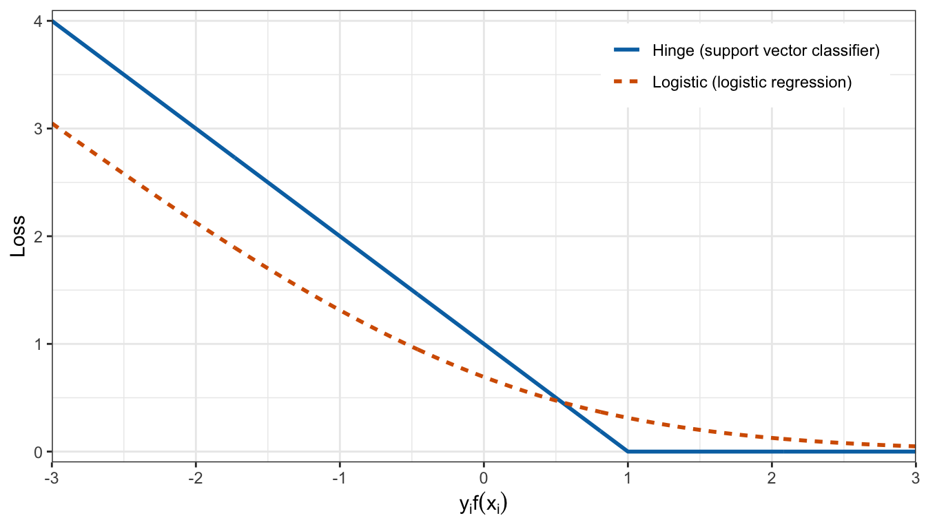
Adding \(\lambda\sum_j w_j^2\) gives ridge-penalized logistic regression. The two classifiers differ only in the loss, a function of \(y_if(x_i)\). The figure plots the two losses against \(y_if(x_i)\).
NoteCode
# Hinge and logistic losses on a grid of y f(x).loss_names <-c("Hinge (support vector classifier)","Logistic (logistic regression)")losses <-tibble(u =seq(-3, 3, by =0.01)) |>mutate(hinge =pmax(0, 1- u),logistic =log(1+exp(-u))) |>pivot_longer(-u, names_to ="loss", values_to ="value") |>mutate(loss =factor(loss, levels =c("hinge", "logistic"),labels = loss_names))loss_plot <-ggplot(losses,aes(x = u, y = value,color = loss, linetype = loss)) +geom_line(linewidth =1) +scale_color_manual(values =c("#0072B2", "#D55E00")) +scale_x_continuous(breaks =seq(-3, 3, by =1),minor_breaks =seq(-2.5, 2.5, by =1)) +scale_y_continuous(breaks =seq(0, 4, by =1),minor_breaks =seq(0.5, 3.5, by =1)) +coord_cartesian(xlim =c(-3, 3), ylim =c(-0.1, 4.1),expand =FALSE) +labs(x =expression(y[i] *f(x[i])), y ="Loss",color =NULL, linetype =NULL) +theme(legend.position ="inside",legend.position.inside =c(0.97, 0.97),legend.justification =c(1, 1))
The two losses have the same shape: large and nearly linear for a misclassified observation, \(y_if(x_i) < 0\), and small for one well on its own side. The hinge loss is exactly 0 from \(y_if(x_i) = 1\) on, so an observation on or outside the margin contributes nothing, and the fit depends only on the support vectors. The logistic loss is positive for every observation, so every observation contributes, the far ones a little. Three differences between the classifiers follow:
Logistic regression estimates a probability \(\Pr(Y = 1 \mid x)\); the support vector classifier gives only a side and a distance, \(\hat f(x)\), with no probability.
When the classes are well separated, the support vector classifier’s boundary is set by the observations near it only, while logistic regression’s estimates are pulled by all of them (and, with perfect separation and no penalty, do not exist).
Kernels apply to logistic regression too, but there every training observation gets a nonzero weight, while the support vector machine’s sum runs over the support vectors only.
32.6.3 Comparison
Logistic regression on the two coordinates, without a penalty, and the linear support vector classifier chosen above, on the same training homes:
# Logistic regression on longitude and latitude, classified at 0.5.logistic_fit <-glm(place ~ longitude + latitude, data = train,family = binomial)p_test <-predict(logistic_fit, test, type ="response")logistic_class <-if_else(p_test >0.5, "Sacramento", "Other")mean(logistic_class != test$place)
[1] 0.221865
On these data the logistic regression’s test error rate, 22.2%, is about the same as that of the linear support vector classifier with cost = 1, 22.5%, and the two classify 99.0% of the test homes the same way. They differ here in both the loss and the penalty, so the comparison does not isolate the loss. The 331 training homes on or outside the support vector classifier’s margin have zero hinge loss and the other 290 positive hinge loss; those 290 and the 2 homes exactly on the margin are its 292 support vectors, which set its fit. The logistic regression gives each test home a probability, which the support vector classifier does not.
NoteBeyond this course
The weights are \(\hat\alpha_i = y_i\hat a_i\), where the multipliers \(0 \le \hat a_i \le \texttt{cost}\) solve the dual of the penalty problem, a quadratic program in one multiplier per observation that involves the data only through \(\langle x_i, x_{i'}\rangle\); so fitting, too, needs only inner products. The Karush-Kuhn-Tucker conditions show that the multiplier is zero for every observation outside the margin. A function can replace the inner product exactly when every matrix \([K(x_i, x_{i'})]\) it produces is positive semidefinite (Mercer’s condition); svm() also offers a sigmoid kernel, and kernels exist for strings, graphs, and other non-numeric data. svm(type = "one-classification") fits a one-class support vector machine for flagging unusual observations. svm(probability = TRUE) fits a logistic curve to the decision values (Platt scaling) to report class probabilities, which are a calibration added after the fit, not part of it. svm() also fits regression (type = "eps-regression"), with a loss that is zero for residuals smaller than \(\epsilon\). See The Elements of Statistical Learning (Hastie, Tibshirani, and Friedman), Sections 12.3 and 12.3.6, or Computer Age Statistical Inference, Chapter 19.
32.7 Conclusion
The support vector classifier fit to polynomial features of the explanatory variables draws a hyperplane in the enlarged feature space, which is a curved boundary in the explanatory variables, but the number of features grows quickly with the number of explanatory variables and the degree. The fitted classifier classifies a new observation through its inner products with the support vectors alone, \(\hat f(x) = \hat w_0 + \sum_{i \in \mathcal{S}}\hat\alpha_i
\langle x, x_i\rangle\). The support vector machine replaces the inner product with a kernel \(K(x, x_i)\): the linear kernel gives back the support vector classifier, the polynomial kernel of degree \(d\) is an inner product of polynomial features computed without listing them, and the radial kernel is local, classifying a new observation by the support vectors near it.
The radial kernel’s \(\gamma\) trades bias against variance: a small \(\gamma\) gives a nearly linear boundary, a large one a boundary that wraps each training observation and overfits. cost and \(\gamma\) are chosen together by cross-validation over a two-dimensional grid with e1071::tune(), and the chosen fit is evaluated by its test error rate and confusion matrix against the linear support vector classifier. With more than two classes, svm() fits one classifier per pair of classes and classifies by vote (one versus one); one versus all fits one classifier per class against the rest.
The support vector classifier minimizes the hinge loss plus a ridge penalty, \(\lambda = 1/(2\,\texttt{cost})\). The hinge loss is zero for observations on or outside the margin, so only the support vectors matter; logistic regression’s loss is positive for every observation and yields probabilities, which the support vector machine does not.
The next lecture begins unsupervised learning with clustering (ISLR2 Chapter 12).