20 Subset Selection

Learning objectives

After this lecture you should be able to

define best subset, forward stepwise, and backward stepwise selection, compare their cost ($2^p$ least squares fits against $1 + p(p+1)/2$), and explain why the stepwise paths need not contain the best model of each size,
explain why the training RSS and $R^2$ cannot choose the number of features $d$ in a model,
derive the $2(d + 1)\sigma^2$ optimism of the training RSS from the covariance between observed and fitted responses, explain why $C_p$ estimates the error on new responses at the observed feature values, and compute $C_p$, BIC, and adjusted $R^2$ for least squares models of each size, stating what each penalizes,
carry out $k$-fold cross-validation of the model size in which the best model of each size is found inside each fold from the training folds only, and compare the size it chooses with the sizes the criteria choose, and
interpret the coefficients of a selected model, including what a dropped dummy variable does to the reference level, and explain why its standard errors and $p$-values are optimistic.

20.1 Used car prices

20.1.1 Data

Question. Which of the recorded explanatory variables should a model of a used car’s price use?

Data. modeldata::car_prices records 804 used General Motors cars for sale in 2005. The response is the price, Price, in dollars. The explanatory variables are the mileage (Mileage), the number of engine cylinders (Cylinder), the number of doors (Doors), indicators of cruise control (Cruise), an upgraded sound system (Sound), and leather seats (Leather), the make (Buick, Cadillac, Chevrolet, Pontiac, Saab, or Saturn), and the body style (convertible, coupe, hatchback, sedan, or wagon). The data store make and body style as one indicator column per level. The tabs plot price against mileage, one panel per make, and against each of the other explanatory variables.

Code

make_names <- c("Buick", "Cadillac", "Chevy", "Pontiac", "Saab", "Saturn")
body_names <- c("convertible", "coupe", "hatchback", "sedan", "wagon")
level_of <- function(data, columns) columns[max.col(as.matrix(data[columns]))]
car_data <- modeldata::car_prices |>
  mutate(make = factor(level_of(modeldata::car_prices, make_names), levels = make_names),
         body = factor(level_of(modeldata::car_prices, body_names), levels = body_names))
n <- nrow(car_data)

violin <- geom_violin(fill = "grey90", scale = "width",
                      quantiles = c(0.25, 0.5, 0.75), quantile.linetype = "solid")
mileage_axis <- scale_x_continuous(labels = scales::label_comma(),
                                   breaks = c(0, 20000, 40000))
mileage_plot <- ggplot(car_data, aes(x = Mileage, y = Price)) +
  geom_point(alpha = 0.4, size = 0.8) +
  facet_wrap(~ make) +
  mileage_axis +
  scale_y_continuous(labels = scales::label_dollar()) +
  labs(x = "Mileage", y = "Price", title = "modeldata::car_prices")

group_levels <- c(make_names, body_names)
group_plot <- bind_rows(
  tibble(variable = "Make", level = as.character(car_data$make), Price = car_data$Price),
  tibble(variable = "Body style", level = as.character(car_data$body), Price = car_data$Price)) |>
  mutate(level = factor(level, levels = group_levels),
         variable = factor(variable, levels = c("Make", "Body style"))) |>
  ggplot(aes(x = level, y = Price)) +
  violin +
  facet_wrap(~ variable, scales = "free_x") +
  scale_y_continuous(labels = scales::label_dollar()) +
  labs(x = NULL, y = "Price", title = "modeldata::car_prices",
       caption = "Lines = quartiles and median.")

option_names <- c("Cylinder", "Doors", "Cruise", "Sound", "Leather")
option_plot <- car_data |>
  mutate(across(c(Cruise, Sound, Leather), \(v) if_else(v == 1, "Yes", "No")),
         across(c(Cylinder, Doors), as.character)) |>
  pivot_longer(all_of(option_names), names_to = "variable", values_to = "level") |>
  mutate(variable = factor(variable, levels = option_names)) |>
  ggplot(aes(x = level, y = Price)) +
  violin +
  facet_wrap(~ variable, scales = "free_x", nrow = 1) +
  scale_y_continuous(labels = scales::label_dollar()) +
  labs(x = NULL, y = "Price", title = "modeldata::car_prices",
       caption = "Lines = quartiles and median.")
# Median price at each level of an explanatory variable, for prose.
median_by <- function(v) tapply(car_data$Price, car_data[[v]], median)

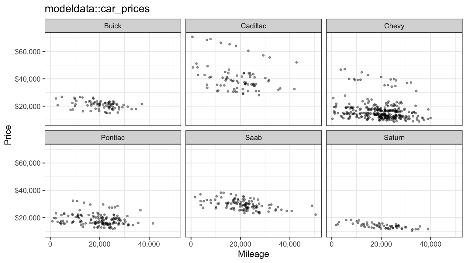
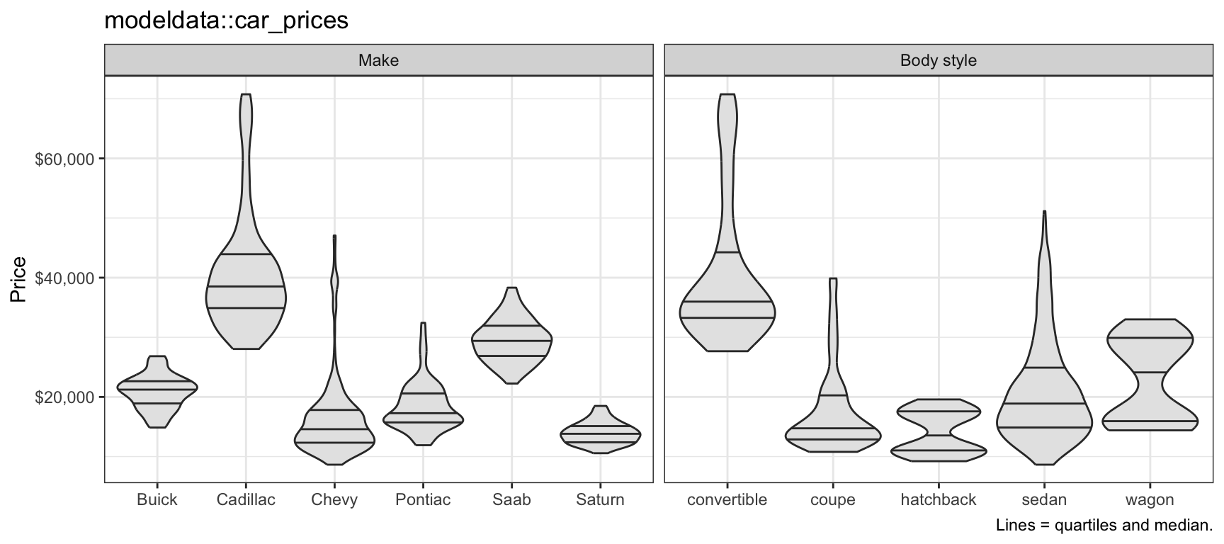
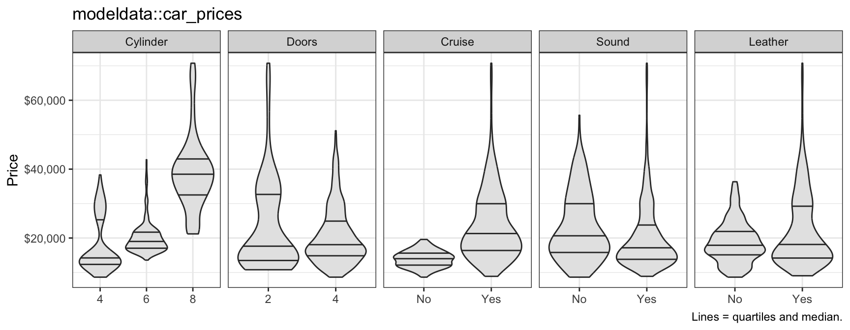
Within every make, price falls with mileage. Make matters more: every Cadillac costs more than every Saturn, and Saab prices sit well above those of Chevrolets and Pontiacs. Convertibles cost the most of the body styles. Cars with more cylinders or with cruise control tend to cost more. Doors and leather seats make little difference to the median price on their own: $17,631 with two doors against $18,073 with four, and $17,895 without leather against $18,126 with it. Cars with an upgraded sound system have a lower median price than cars without one, $17,161 against $20,648; Chevrolets, the most common make and one of the cheapest, have one 82.8% of the time. Prices spread more widely where they are higher: the Cadillac panel spans a far wider range of dollars than the Saturn panel.

20.1.2 Candidate features

The first five explanatory variables enter as features as recorded, with Cylinder treated as a number (4, 6, or 8). Make and body style are categorical explanatory variables, and their indicator columns are complete sets: every car has exactly one make and one body style, so the six make indicators sum to 1, the intercept column. Each needs a reference level whose indicator is left out; here Saturn for make and wagon for body style.

doors_from_body <- all(car_data$Doors == 4 - 2 * (car_data$convertible + car_data$coupe))

Doors is redundant as well. Every convertible and coupe has two doors and every other car four, so $\texttt{Doors} = 4 - 2\left(\texttt{convertible} + \texttt{coupe}\right)$ for every car (doors_from_body is TRUE), and with the body style indicators in the model Doors would be an exact linear combination of other columns. It is dropped.

features <- c("Mileage", "Cylinder", "Cruise", "Sound", "Leather",
              setdiff(make_names, "Saturn"), setdiff(body_names, "wagon"))
p <- length(features)

That leaves $p = 14$ candidate features, and the largest model is

\[y_i = \beta_0 + \beta_1 x_{i1} + \cdots + \beta_p x_{ip} + \epsilon_i, \qquad \epsilon_i \stackrel{ind}{\sim} N\left(0, \sigma^2\right),\]

where

$y_i$ is the response for car $i = 1, \ldots, n$, with $n = 804$: its price or, as decided next, the logarithm of its price,
$x_{ij}$ is the value of feature $j = 1, \ldots, p$ for car $i$, in the order Mileage, Cylinder, Cruise, Sound, Leather, Buick, Cadillac, Chevy, Pontiac, Saab, convertible, coupe, hatchback, and sedan, and $x_i = \left(1, x_{i1}, \ldots, x_{ip}\right)$ is row $i$ of the model matrix $\mathbf{X}$,
$\beta_0, \ldots, \beta_p$ are the coefficients, and
$\epsilon_i$ is the error, with variance $\sigma^2$.

A subset of the features is a smaller model of the same form with the coefficients of the other features set to zero.

20.1.3 Price scale

Code

cars <- car_data |>
  transmute(log_price = log(Price), across(all_of(features)))
full_dollars <- lm(Price ~ ., data = select(car_data, Price, all_of(features)))
full_log <- lm(log_price ~ ., data = cars)
spread_cor <- c(dollars = cor(abs(residuals(full_dollars)), fitted(full_dollars)),
                log = cor(abs(residuals(full_log)), fitted(full_log)))

residual_plot <- function(fit, x_label, y_label, scale_name) {
  ggplot(tibble(fitted = fitted(fit), residual = residuals(fit)),
         aes(x = fitted, y = residual)) +
    geom_hline(yintercept = 0, color = "grey50") +
    geom_point(alpha = 0.4, size = 0.8) +
    labs(x = x_label, y = y_label,
         title = paste("All", p, "features, price", scale_name))
}
residual_plots <- list(
  residual_plot(full_dollars, "Fitted price ($)", "Residual ($)", "in dollars") +
    scale_x_continuous(labels = scales::label_comma()) +
    scale_y_continuous(labels = scales::label_comma()),
  residual_plot(full_log, "Fitted log price", "Residual (log scale)", "on the log scale"))

The tabs plot the residuals against the fitted values of the largest model, fit by least squares once with price in dollars as the response and once with its natural logarithm.

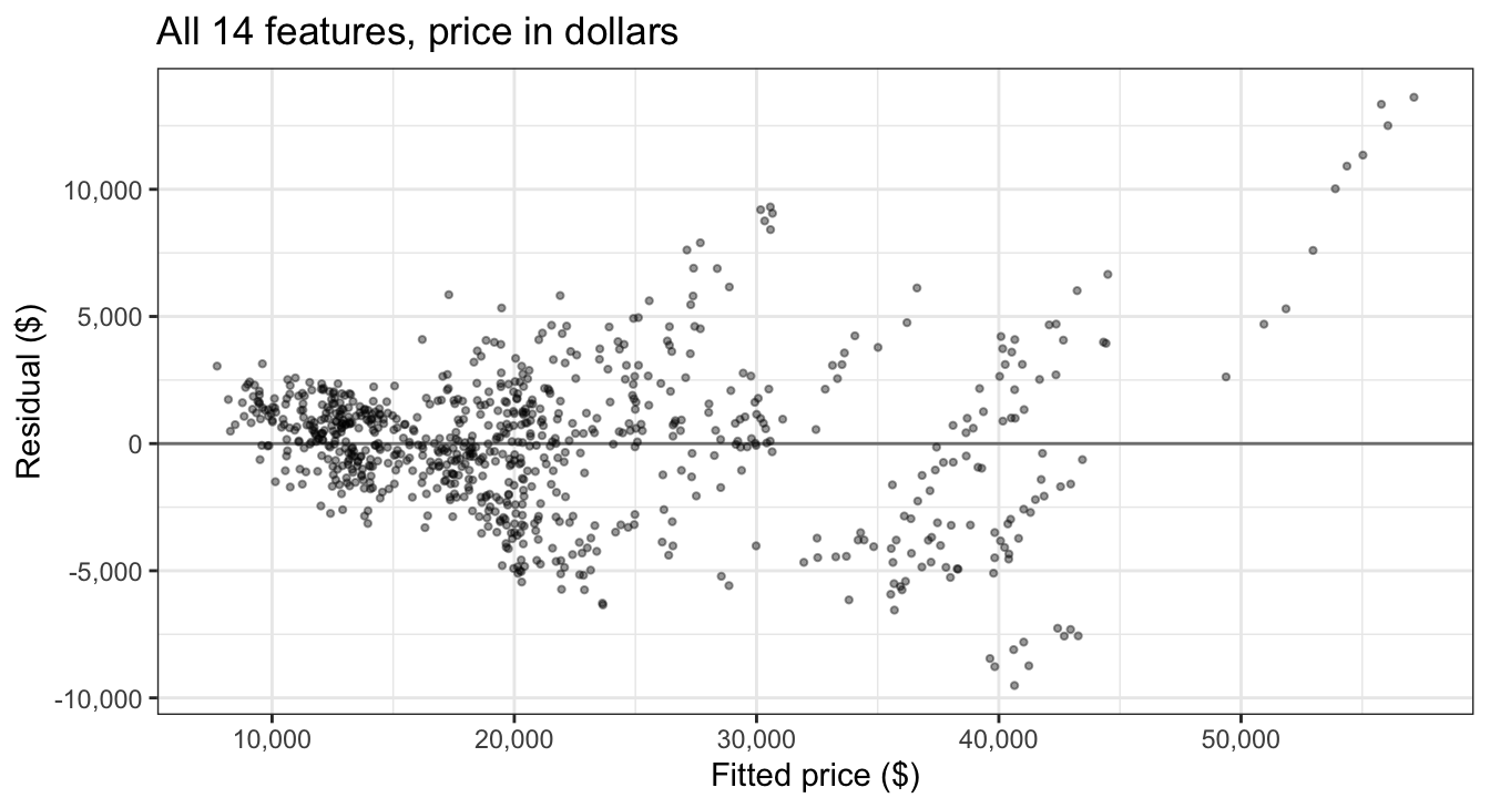
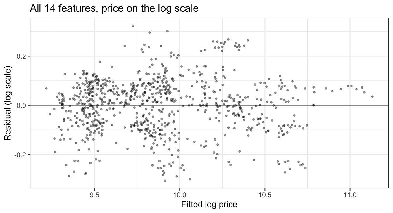
In dollars the residuals fan out as the fitted price rises: the correlation between the absolute residual and the fitted value is 0.56. On the log scale it is 0.11, close to the constant variance the model assumes. Errors of similar size on the log scale are errors of similar percentage in price, which matches prices that vary by a few thousand dollars for a Saturn and by many thousands for a Cadillac. From here on the response is $y_i = \log\left(\texttt{Price}_i\right)$. The largest model explains $R^2 = 92.9\%$ of the variability in log price, with $\hat\sigma = 0.1103$.

20.1.4 Selection motives

The largest model fits well, so why use fewer features?

Interpretability. A model with fewer features is easier to explain, and each coefficient that is truly zero but estimated anyway adds noise to the story the model tells.
Variance. Least squares fitted values are $\hat y = \mathbf{H}y$ with $\mathbf{H} = \mathbf{X}\left(\mathbf{X}^\top\mathbf{X}\right)^{-1}\mathbf{X}^\top$, so $Var\left[\hat y\right] = \sigma^2\mathbf{H}\mathbf{H}^\top = \sigma^2\mathbf{H}$. Its trace is $\sigma^2\,\text{tr}(\mathbf{H}) = \sigma^2(d + 1)$ for a model with $d$ features and an intercept, so

\[\frac{1}{n}\sum_{i=1}^n Var\left[\hat y_i\right] = \frac{\sigma^2(d+1)}{n},\]

where $d$ is the number of features in the model, its size, and $\text{tr}$ is the trace. In the Cross-Validation lecture $d$ was the degree of a polynomial; a degree-$d$ polynomial has $d$ features, so the two meanings agree there. Every feature added raises the average variance of the fitted values by $\sigma^2/n$, whether or not its true coefficient is zero; it lowers the bias only if its coefficient is not zero. With $n = 804$ and $p = 14$ the cost is small here, and it grows as $p$ approaches $n$.
Search. Each feature is either in or out, so there are $2^p$ candidate models, $2^{14} = 16,384$ for these cars.

20.2 Best subset selection

The figure plots log price (on a dollar axis) against mileage, one panel per make, the view of the data the models below will be drawn on.

Code

log_price_axis <- scale_y_log10(breaks = c(10, 15, 20, 30, 40, 60) * 1000,
                                labels = scales::label_dollar(accuracy = 1))
log_base <- ggplot(car_data, aes(x = Mileage, y = Price)) +
  geom_point(color = "grey55", alpha = 0.5, size = 0.8) +
  facet_wrap(~ make) +
  mileage_axis +
  log_price_axis +
  labs(x = "Mileage", y = "Price (log scale)", title = "modeldata::car_prices")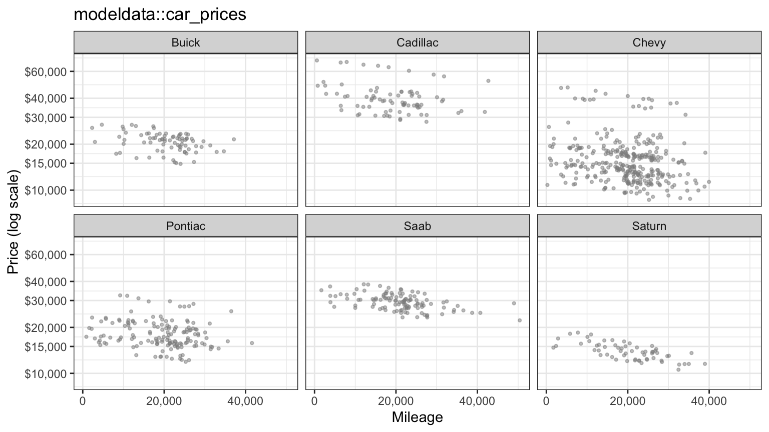

Within a make the cars form bands at different price levels, cars that differ in engine size and in other unrecorded ways, and within a band price falls with mileage.

20.2.1 Algorithm

Best subset selection fits every subset:

Let $\mathcal{M}_0$ be the null model, with no features, which predicts $\bar y$ for every car.
For $d = 1, \ldots, p$, fit all $\binom{p}{d}$ models with exactly $d$ features by least squares, and let $\mathcal{M}_d$ be the one with the smallest RSS, equivalently the largest $R^2$.
Choose one model among $\mathcal{M}_0, \ldots, \mathcal{M}_p$ with an estimate of the error on new data: $C_p$, BIC, adjusted $R^2$, or cross-validation.

Here $\mathcal{M}_d$ is the best model of size $d$, and $RSS_d$ is its residual sum of squares. Step 2 compares models of the same size, and for them the training RSS is a fair comparison: each has the same number of coefficients to fit with. Step 3 compares models of different sizes, which is where training error fails. The number of models fit is $\sum_{d=0}^p\binom{p}{d} = 2^p$.

20.2.2 Fitting

leaps::regsubsets() carries out step 2. The argument nvmax is the largest size to search.

best_fit <- regsubsets(log_price ~ ., data = cars, nvmax = p, method = "exhaustive")
best_summary <- summary(best_fit)

Code

# Feature-by-size inclusion matrix, without the intercept column.
best_which <- best_summary$which[, -1]
features_of <- function(which_matrix, d) colnames(which_matrix)[which_matrix[d, ]]
nested <- all(map_lgl(2:p, \(d) all(best_which[d - 1, ] <= best_which[d, ])))
entry_size <- apply(best_which, 2, \(included) min(which(included)))
entry_order <- names(sort(entry_size))

which_plot <- function(which_matrix, title) {
  as_tibble(which_matrix) |>
    mutate(d = row_number()) |>
    pivot_longer(-d, names_to = "feature", values_to = "included") |>
    mutate(feature = factor(feature, levels = rev(entry_order))) |>
    ggplot(aes(x = d, y = feature, fill = included)) +
    geom_tile(color = "grey70") +
    scale_fill_manual(values = c(`FALSE` = "white", `TRUE` = "grey20"),
                      labels = c("Out", "In")) +
    scale_x_continuous(breaks = seq_len(p), expand = c(0, 0)) +
    labs(x = "Model size d", y = NULL, fill = NULL, title = title)
}
best_which_plot <- which_plot(best_which, "Best subset of each size, all cars")

show_sizes <- 1:4
fitted_plots <- map(show_sizes, \(d) {
  fit <- lm(reformulate(features_of(best_which, d), "log_price"), data = cars)
  log_base +
    geom_point(data = mutate(car_data, Price = exp(fitted(fit))),
               color = "#D55E00", shape = 4, size = 0.9) +
    labs(subtitle = paste0("Fitted values (crosses) of the best model with ", d,
                           if (d == 1) " feature: " else " features: ",
                           paste(features_of(best_which, d), collapse = " + ")))
})

The tabs add the fitted values of the best models with 1, 2, 3, and 4 features to the plot above.

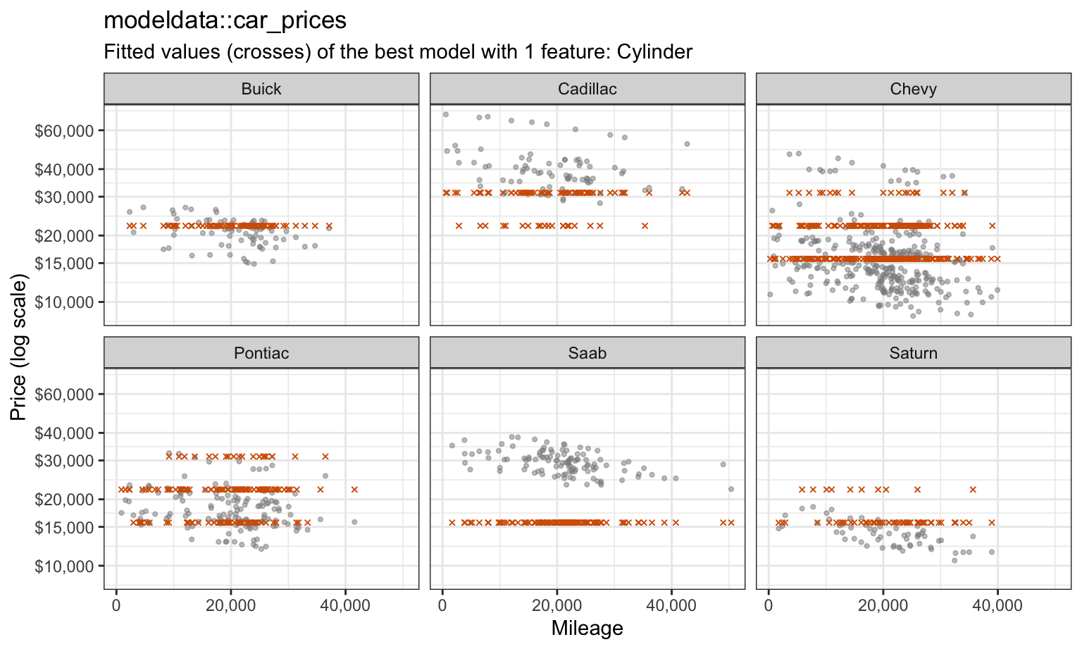
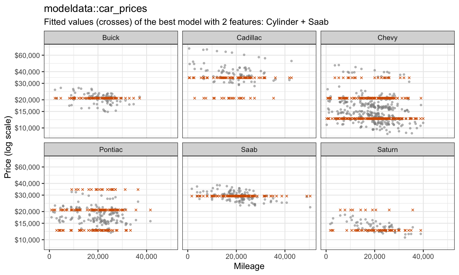
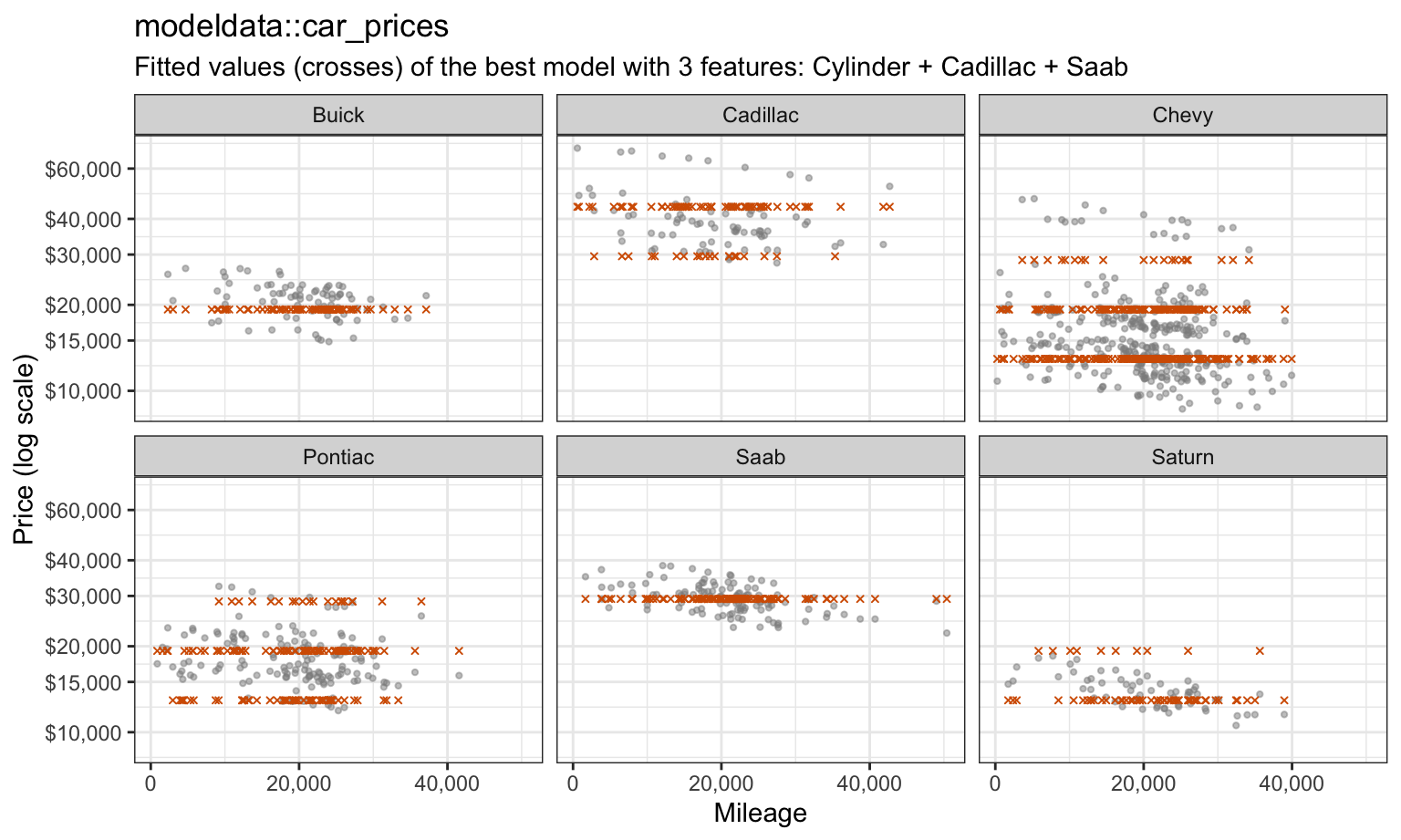
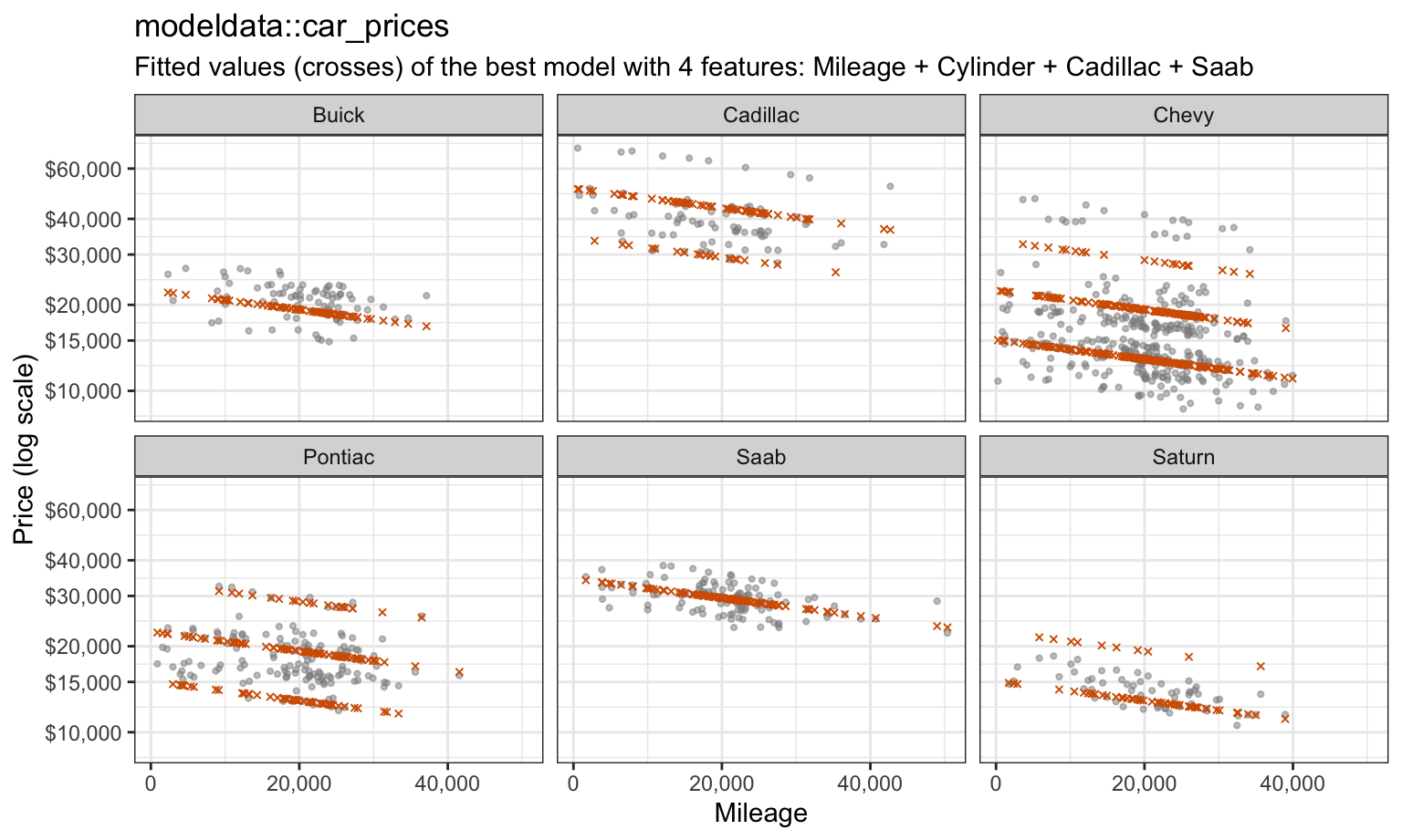
The best single feature is Cylinder, which gives one fitted level per engine size and leaves Saabs, all four-cylinder cars, far below their prices. The best pair adds Saab, which lifts every Saab; the best triple adds Cadillac; and only at size 4 does Mileage enter, tilting each band downward. The figure below shows the features in the best model of every size.

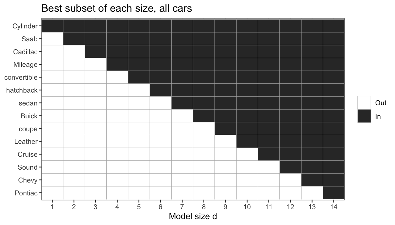
On these data the best models are nested: each contains the best model one size smaller (nested is TRUE). Nothing in the algorithm requires that, since each size is searched separately.

20.2.3 Training RSS

Code

X <- model.matrix(log_price ~ ., data = cars)
y <- cars$log_price
tss <- sum((y - mean(y))^2)
# RSS of all 2^p subsets; column 1 of X is the intercept.
all_subsets <- map(0:p, \(d) {
  sets <- if (d == 0) list(integer(0)) else combn(p, d, simplify = FALSE)
  tibble(d = d, rss = map_dbl(sets, \(s) sum(lm.fit(X[, c(1, s + 1), drop = FALSE], y)$residuals^2)))
}) |>
  list_rbind()
best_rss <- all_subsets |>
  group_by(d) |>
  summarize(rss = min(rss), .groups = "drop")
rss_decreasing <- all(diff(best_rss$rss) < 0)

rss_plot <- ggplot(all_subsets, aes(x = d, y = rss)) +
  # A fixed jitter seed for this one figure, so drawing it leaves the
  # chapter's random number stream (and every later result) unchanged.
  geom_point(color = "grey60", alpha = 0.15, size = 0.8,
             position = position_jitter(width = 0.15, height = 0, seed = 1)) +
  geom_line(data = best_rss) +
  geom_point(data = best_rss, size = 2) +
  scale_x_continuous(breaks = 0:p) +
  scale_y_continuous(sec.axis = sec_axis(~ 1 - . / tss, name = expression(R^2))) +
  labs(x = "Model size d", y = "Training RSS",
       title = paste("All", format(2^p, big.mark = ","), "subsets; best of each size in black"))

The figure plots the training RSS of all 16,384 subsets against their size, with the best of each size, $RSS_d$, joined by the black line. $R^2 = 1 - RSS/TSS$ is a decreasing function of RSS, so the right axis reads off the same points as $R^2$.

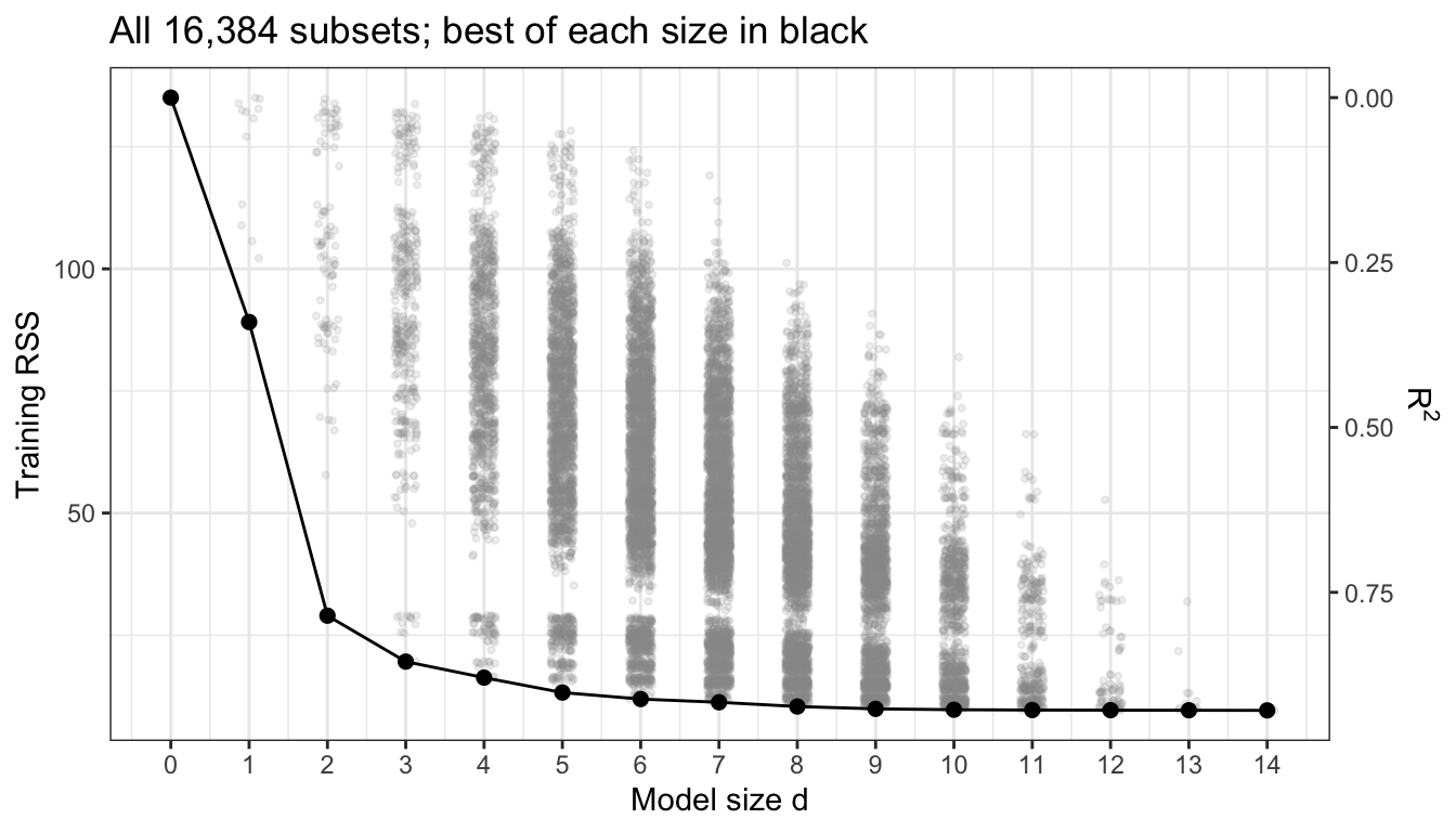
$RSS_d$ falls at every step, from $RSS_0 = TSS = 135.06$ to 89.11 at $d = 1$ and 9.60 at $d = 14$ (rss_decreasing is TRUE). It cannot do otherwise. Adding any feature to $\mathcal{M}_d$ gives a model of size $d + 1$ whose least squares fit can match $\mathcal{M}_d$ by setting the new coefficient to zero, so $RSS_{d+1} \le RSS_d$. The training RSS and $R^2$ therefore always choose $d = p$. This is the argument the Cross-Validation lecture made for polynomial degree: training error rewards every addition, whether or not it will help predict new cars.

20.2.4 Computational cost

The 16,384 least squares fits above take a few seconds. The count doubles with each candidate feature: $2^{20}$ is about a million, $2^{30}$ about a billion, and $2^{40}$ about a trillion. The size of the search has a statistical cost too. The Cross-Validation in Practice lecture showed that the smallest of many noisy estimates tends to be optimistic, and the more subsets searched, the more likely one of them fits the noise in these particular cars well.

20.3 Stepwise selection

The figure shows the correlation between every pair of features and with log price.

Code

cor_cars <- cor(cars)
cor_labels <- c(log_price = "log(Price)")
display_name <- function(v) if_else(v %in% names(cor_labels), cor_labels[v], v)
cor_plot <- as_tibble(cor_cars, rownames = "row") |>
  pivot_longer(-row, names_to = "column", values_to = "r") |>
  mutate(row = factor(display_name(row), levels = display_name(names(cars))),
         column = factor(display_name(column), levels = rev(display_name(names(cars))))) |>
  ggplot(aes(x = row, y = column, fill = r)) +
  geom_tile() +
  geom_text(aes(label = sprintf("%.2f", r)), size = 2.2) +
  scale_fill_gradient2(low = "#0072B2", mid = "white", high = "#D55E00",
                       limits = c(-1, 1)) +
  labs(x = NULL, y = NULL, fill = "Correlation", title = "modeldata::car_prices") +
  theme(axis.text.x = element_text(angle = 45, hjust = 1))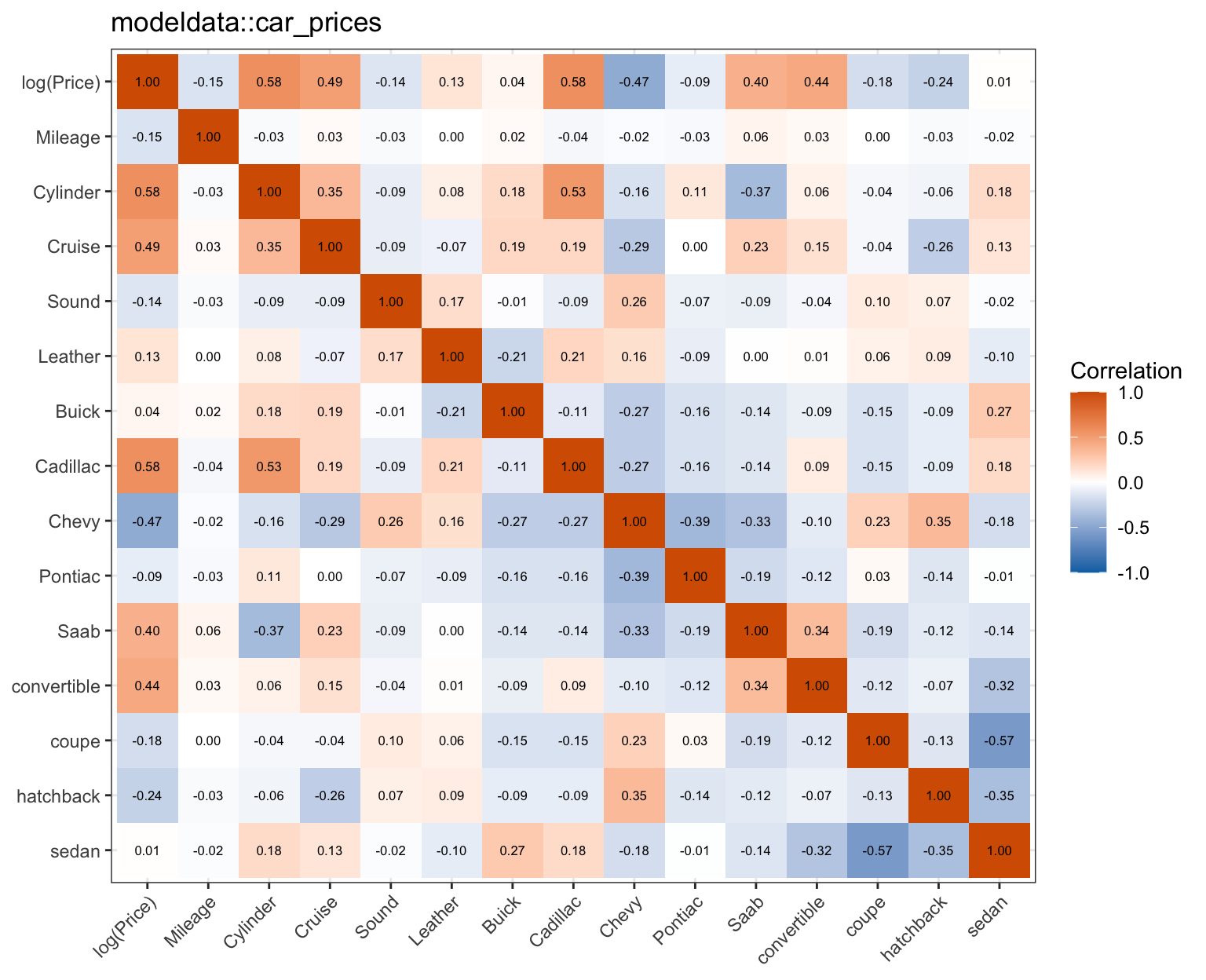

Cylinder and Cadillac are the two features most correlated with log price, 0.58 and 0.58, and with each other, 0.53: Cadillacs mostly have eight cylinders. Saab is negatively correlated with Cylinder, -0.37, because every Saab has four cylinders, and positively with log price. Features that overlap like this can substitute for each other, which is where a search that adds or removes one feature at a time can go astray.

20.3.1 Forward stepwise

Forward stepwise selection grows one model:

Let $\mathcal{M}_0$ be the null model.
For $d = 0, \ldots, p - 1$, fit the $p - d$ models that add one feature to $\mathcal{M}_d$, and let $\mathcal{M}_{d+1}$ be the one with the smallest RSS.
Choose one model among $\mathcal{M}_0, \ldots, \mathcal{M}_p$ as in best subset selection.

The number of models fit is

\[1 + \sum_{d=0}^{p-1}(p - d) = 1 + \frac{p(p+1)}{2},\]

106 for $p = 14$, against 16,384 for best subset selection. Forward stepwise needs only $d < n$ for each model it fits, so it can be used when $p \ge n$, stopping at size $n - 1$.

20.3.2 Backward stepwise

Backward stepwise selection shrinks one model:

Let $\mathcal{M}_p$ be the model with all $p$ features.
For $d = p, \ldots, 1$, fit the $d$ models that remove one feature from $\mathcal{M}_d$, and let $\mathcal{M}_{d-1}$ be the one with the smallest RSS.
Choose one model among $\mathcal{M}_0, \ldots, \mathcal{M}_p$ as before.

It fits the same $1 + p(p+1)/2$ models, but it starts from the full least squares fit, so it needs $n > p$.

Both are greedy: forward never removes a feature it has added, and backward never restores one it has removed, so their models are nested by construction. The best model of size $d$ need not contain the best model of size $d - 1$, and when it does not, a stepwise path misses it.

20.3.3 Path comparison

forward_fit <- regsubsets(log_price ~ ., data = cars, nvmax = p, method = "forward")
backward_fit <- regsubsets(log_price ~ ., data = cars, nvmax = p, method = "backward")
same_forward <- identical(summary(forward_fit)$which, best_summary$which)
same_backward <- identical(summary(backward_fit)$which, best_summary$which)

On all 804 cars the three methods give identical models at every size (same_forward is TRUE and same_backward is TRUE), because the best models happen to be nested. That is a property of these data, not of the methods.

Code

n_halves <- 200
methods <- c("exhaustive", "forward", "backward")
method_labels <- c(exhaustive = "Best subset", forward = "Forward", backward = "Backward")
halves <- map(seq_len(n_halves), \(r) {
  id <- sample(n, n / 2)
  fits <- map(methods, \(m) summary(regsubsets(log_price ~ ., data = cars[id, ],
                                               nvmax = p, method = m)))
  names(fits) <- methods
  list(id = id, fits = fits,
       differs = map(fits[-1], \(f) rowSums(f$which != fits$exhaustive$which) > 0))
})
share_forward <- mean(map_lgl(halves, \(h) any(h$differs$forward)))
share_backward <- mean(map_lgl(halves, \(h) any(h$differs$backward)))
share_forward_2 <- mean(map_lgl(halves, \(h) h$differs$forward[2]))

# The first half in which forward stepwise misses the best pair of features.
example <- halves[[which(map_lgl(halves, \(h) h$differs$forward[2]))[1]]]
cell <- function(f, d) {
  paste0(paste(colnames(f$which)[f$which[d, ]][-1], collapse = " + "),
         " (", fmt(f$rss[d]), ")")
}
example_table <- map(methods, \(m) {
  tibble(Method = method_labels[[m]], d1 = cell(example$fits[[m]], 1),
         d2 = cell(example$fits[[m]], 2), d3 = cell(example$fits[[m]], 3))
}) |>
  list_rbind() |>
  knitr::kable(col.names = c("Method", "Size 1 (RSS)", "Size 2 (RSS)", "Size 3 (RSS)"))
ex_rss <- function(m, d) example$fits[[m]]$rss[d]
ex_features <- function(m, d) colnames(example$fits[[m]]$which)[example$fits[[m]]$which[d, ]][-1]
single_rss <- map_dbl(c("Cylinder", "Cadillac"),
                      \(f) sum(residuals(lm(reformulate(f, "log_price"), data = cars))^2))

To see how often the paths differ, the three methods were run on 200 random halves of the cars. Forward stepwise differs from best subset at one or more sizes in 72.5% of the halves, and backward stepwise in 72.5%. The table shows the first three models of each method in one half where they differ, with each model’s training RSS on that half.

Method	Size 1 (RSS)	Size 2 (RSS)	Size 3 (RSS)
Best subset	Cadillac (44.51)	Cylinder + Saab (14.51)	Cylinder + Cadillac + Saab (9.56)
Forward	Cadillac (44.51)	Cadillac + Saab (27.51)	Cylinder + Cadillac + Saab (9.56)
Backward	Cylinder (45.52)	Cylinder + Saab (14.51)	Cylinder + Cadillac + Saab (9.56)

In this half Cadillac alone has a slightly smaller RSS than any other single feature, so forward stepwise keeps it, and its best pair, Cadillac + Saab, has RSS 27.51, against 14.51 for the best pair, Cylinder + Saab, which does not contain the best single feature. Backward stepwise reaches the best pair from above and then keeps Cylinder at size 1. On all the cars the single-feature models are close too: Cylinder alone has RSS 89.11 and Cadillac alone 89.62. Forward stepwise misses the best pair in 45.5% of the halves.

Beyond this course

Branch and bound. regsubsets(method = "exhaustive") does not fit all $2^p$ subsets: it uses the fact that removing features can only raise the RSS to rule out whole branches of subsets without fitting them, which makes exact best subset search practical up to a few dozen features.
Hybrid and floating searches. Stepwise variants that, after each addition, consider removing a feature added earlier (or the reverse) recover some of the models a purely greedy path misses.
Mixed-integer optimization. Modern integer-programming solvers can find best subsets for hundreds of features.
Other models. The same three algorithms apply to logistic or Poisson regression, with the deviance in place of the RSS.

20.4 Model size

All three methods leave the same decision: which of $\mathcal{M}_0, \ldots, \mathcal{M}_p$ to use. In this chapter all 804 cars are training data. None are held out as test data, as they are in the test data workflow of the Cross-Validation in Practice lecture, so every estimate of error below comes from the same cars that choose the model.

Code

sigma2_full <- sigma(full_log)^2
train_mse <- tibble(d = 0:p, mse = best_rss$rss / n)
below_from <- min(which(train_mse$mse < sigma2_full)) - 1
zoom_from <- 6
train_mse_plot <- ggplot(filter(train_mse, d >= zoom_from), aes(x = d, y = mse)) +
  geom_hline(yintercept = sigma2_full, linetype = "dashed", color = "grey40") +
  annotate("text", x = p, y = sigma2_full, vjust = -0.6, hjust = 1, size = 3.2,
           label = paste0("Estimated error variance, ", fmt(sigma2_full, 5))) +
  geom_line() +
  geom_point(size = 2) +
  scale_x_continuous(breaks = zoom_from:p) +
  labs(x = "Model size d", y = "Training MSE (log price)",
       title = paste0("Best subset of each size, sizes ", zoom_from, " to ", p))

The figure plots the training MSE, $RSS_d/n$, of the best model of each size from $d = 6$ to $p$, with a dashed line at the estimate of the error variance $\sigma^2$ from the largest model, $\hat\sigma^2 = RSS_p/(n - p - 1) = 0.01216$.

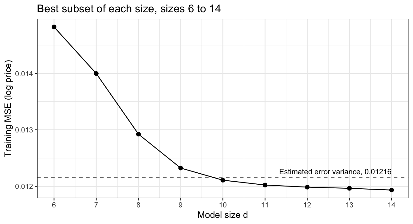
The training MSE is below $\hat\sigma^2$ from $d = 10$ on, and equals 0.01193 at $d = p$. A new car’s log price varies about its mean with variance $\sigma^2$, so no model’s average squared error on new responses can be below $\sigma^2$; the training MSE of the larger models is below an estimate of it. The training error cannot choose the size. There are two ways to estimate the error on new data instead: adjust the training error for the size of the model, or estimate the error directly by cross-validation.

20.4.1 Training error optimism

Fix a least squares model with $d$ features, and imagine new responses $y_i^0$ at the same feature values $x_i$, independent of $y$ with the same distribution. Write $f_i = E\left[y_i\right]$. Since $E\left[y_i^0 - f_i\right] = 0$ and $y_i^0$ is independent of $\hat y_i$,

\[E\left[\left(y_i^0 - \hat y_i\right)^2\right] = \sigma^2 + E\left[\left(\hat y_i - f_i\right)^2\right], \qquad E\left[\left(y_i - \hat y_i\right)^2\right] = \sigma^2 + E\left[\left(\hat y_i - f_i\right)^2\right] - 2\,Cov\left[y_i, \hat y_i\right].\]

The training residual is smaller because $\hat y_i$ was fit to $y_i$. With $\hat y_i = \sum_j h_{ij}y_j$ and independent errors, $Cov\left[y_i, \hat y_i\right] = h_{ii}\sigma^2$, and summing over $i$,

\[E\left[\sum_{i=1}^n\left(y_i^0 - \hat y_i\right)^2\right] = E\left[RSS\right] + 2\sigma^2\,\text{tr}(\mathbf{H}) = E\left[RSS\right] + 2(d+1)\sigma^2,\]

where $y_i^0$ is a new response at $x_i$, $f_i$ its mean, and $h_{ij}$ the $(i, j)$ entry of the hat matrix $\mathbf{H}$. The training RSS underestimates the error on new responses at the same $x_i$ by $2(d+1)\sigma^2$ on average, an amount that grows with the size of the model. For the largest model of the figure above, $2(p + 1)\hat\sigma^2/n = 0.00045$ lifts the training MSE of 0.01193 to 0.01239, above $\hat\sigma^2$.

20.4.2 Penalized criteria

Adding that penalty back gives

\[C_p = \frac{1}{n}\left(RSS + 2d\hat\sigma^2\right), \qquad \text{BIC} = \frac{1}{n}\left[RSS + \log(n)\,d\hat\sigma^2\right], \qquad \text{Adjusted } R^2 = 1 - \frac{RSS/(n - d - 1)}{TSS/(n - 1)},\]

where

$RSS$ is the training residual sum of squares of the model and $d$ its number of features,
$\hat\sigma^2$ is an estimate of the error variance from the model with all $p$ features, the same for every size, which keeps the larger models from estimating their own (smaller) error variance,
$TSS = \sum_{i=1}^n\left(y_i - \bar y\right)^2$ is the total sum of squares, and
$\log$ is the natural logarithm. The subscript $p$ in $C_p$ is Mallows’ historical name, not the number of features.

$C_p$ is $RSS/n$ plus the optimism above divided by $n$, with $2d$ in place of $2(d+1)$; the difference, $2\hat\sigma^2/n$, is the same at every size and does not change which size wins. If $\hat\sigma^2$ is unbiased for $\sigma^2$, then for a model fixed in advance $E\left[C_p\right] + 2\sigma^2/n = E\left[\frac{1}{n}\sum_{i=1}^n\left(y_i^0 - \hat y_i\right)^2\right]$: up to the constant $2\sigma^2/n$, $C_p$ estimates the average error on new responses at the observed feature values $x_1, \ldots, x_n$. Choose the size with the smallest $C_p$ or BIC, or the largest adjusted $R^2$.

The AIC and BIC come from the likelihood. With $\epsilon_i \stackrel{ind}{\sim} N\left(0, \sigma^2\right)$ and $\sigma^2$ fixed at $\hat\sigma^2$, the maximized log-likelihood is $\log L = -\frac{n}{2}\log\left(2\pi\hat\sigma^2\right) - RSS/\left(2\hat\sigma^2\right)$, and

\[\text{AIC} = -2\log L + 2(d+1), \qquad \text{BIC} = -2\log L + \log(n)(d+1).\]

Multiplying by $\hat\sigma^2/n$ and dropping the terms that do not depend on $d$, among them the intercept’s share of each penalty ($2\hat\sigma^2/n$ in the AIC), leaves $C_p$ and the BIC above, so for least squares with Gaussian errors AIC and $C_p$ choose the same size.

Each criterion trades a drop in RSS against a penalty per feature. Going from $\mathcal{M}_d$ to $\mathcal{M}_{d+1}$ lowers $C_p$ if $\left(RSS_d - RSS_{d+1}\right)/\hat\sigma^2 > 2$ and lowers the BIC if it exceeds $\log(n) = 6.69$. Adjusted $R^2$ rises if $RSS_{d+1}/(n - d - 2) < RSS_d/(n - d - 1)$, which rearranges to

\[F = \frac{RSS_d - RSS_{d+1}}{RSS_{d+1}/(n - d - 2)} > 1,\]

the $F$-statistic of the multiple regression lecture for the added feature. For $n > 7$, $\log(n) > 2$, so the BIC penalizes each feature more than $C_p$ and tends to choose smaller models; adjusted $R^2$, with a threshold of 1 and the error variance of the larger model in the denominator, penalizes least.

rss <- best_summary$rss
sizes <- seq_len(p)
sigma2_hat <- sigma(full_log)^2
criteria <- tibble(d = sizes,
                   Cp = (rss + 2 * d * sigma2_hat) / n,
                   BIC = (rss + log(n) * d * sigma2_hat) / n,
                   adj_R2 = 1 - (rss / (n - d - 1)) / (tss / (n - 1)))
d_cp <- which.min(criteria$Cp)
d_bic <- which.min(criteria$BIC)
d_adj <- which.max(criteria$adj_R2)

On the cars, with $\hat\sigma^2 = 0.01216$, $C_p$ chooses $d = 12$, the BIC $d = 10$, and adjusted $R^2$ $d = 14$. The derivation holds for a model fixed in advance; $\mathcal{M}_d$ was chosen as the best of $\binom{p}{d}$ fits, so its RSS is lower than a fixed model’s would be, and all three criteria share some of the selection optimism of the Cross-Validation in Practice lecture.

20.4.3 Within-fold cross-validation

Cross-validation estimates the error of each size on new cars directly. The rule of the Cross-Validation and Cross-Validation in Practice lectures applies: every data-dependent step of the fit is repeated inside each fold, using only the training folds. Here step 2 of best subset selection is a data-dependent step. Within fold $\ell$, the best model of each size is found from the training folds and then used to predict the validation fold, the held-out fold $\ell$. Running best subset selection once on all 804 cars and cross-validating only the coefficients would let the held-out cars help choose the features that predict them.

regsubsets() has no predict() method, so predict_subset() multiplies the model matrix of new cars by the coefficients of the best model of size d.

predict_subset <- function(fit, new_data, d) {
  b <- coef(fit, id = d)
  X_new <- model.matrix(log_price ~ ., data = new_data)
  drop(X_new[, names(b), drop = FALSE] %*% b)
}
cv_by_size <- function(data, fold) {
  sq_error <- matrix(NA_real_, nrow(data), p)
  for (l in unique(fold)) {
    held_out <- fold == l
    # Best subset of every size, from the training folds only.
    fold_fit <- regsubsets(log_price ~ ., data = data[!held_out, ], nvmax = p)
    for (d in seq_len(p)) {
      sq_error[held_out, d] <- (data$log_price[held_out] -
                                  predict_subset(fold_fit, data[held_out, ], d))^2
    }
  }
  colMeans(sq_error)
}
n_folds <- 10
fold_cars <- sample(rep(seq_len(n_folds), length.out = n))
cv_mse <- cv_by_size(cars, fold_cars)
d_cv <- which.min(cv_mse)

$\text{CV}_{(k)}(d)$, the $k$-fold estimate with $k = 10$, estimates the test MSE of the procedure “fit the best model of size $d$”, not of one fixed set of features: the best model of a size can differ from fold to fold. The number of folds $k$ is unrelated to the $K$ of KNN or the number of classes $K$.

Code

# How often the best model of a size in a fold differs from the one on all cars.
fold_differs <- map(seq_len(n_folds), \(l) {
  w <- summary(regsubsets(log_price ~ ., data = cars[fold_cars != l, ], nvmax = p))$which
  rowSums(w != best_summary$which) > 0
}) |>
  do.call(what = rbind)
share_fold_differs <- mean(fold_differs)
sizes_fold_differs <- sizes[colSums(fold_differs) > 0]

# The chosen size over further random partitions into folds.
n_partitions <- 20
partition_sizes <- map_int(seq_len(n_partitions), \(r) {
  which.min(cv_by_size(cars, sample(rep(seq_len(n_folds), length.out = n))))
})
partition_counts <- count(tibble(d = partition_sizes), d)

In these folds the best model of a size differs from the one found on all the cars in 7.1% of the fold-and-size combinations, at sizes 1, 4, and 7. Cross-validation chooses $d = 13$, with $\text{CV}_{(10)} = 0.01233$.

20.4.4 Chosen sizes

Code

mse_labels <- c("Cp", "BIC", paste0(n_folds, "-fold CV"))
mse_criteria <- bind_rows(
  tibble(d = sizes, value = criteria$Cp, criterion = mse_labels[1]),
  tibble(d = sizes, value = criteria$BIC, criterion = mse_labels[2]),
  tibble(d = sizes, value = cv_mse, criterion = mse_labels[3])) |>
  mutate(criterion = factor(criterion, levels = mse_labels))
chosen <- tibble(criterion = factor(mse_labels, levels = mse_labels),
                 d = c(d_cp, d_bic, d_cv)) |>
  left_join(mse_criteria, by = c("criterion", "d"))
criterion_colors <- setNames(c("#0072B2", "#D55E00", "#009E73"), mse_labels)
mse_plot <- function(from_d) {
  shown <- filter(mse_criteria, d >= from_d)
  ggplot(shown, aes(x = d, y = value, color = criterion, linetype = criterion,
                    shape = criterion)) +
    geom_line() +
    geom_point(size = 1.8) +
    geom_point(data = chosen, size = 5, stroke = 1.2, show.legend = FALSE) +
    scale_x_continuous(breaks = from_d:p) +
    scale_color_manual(values = criterion_colors) +
    scale_shape_manual(values = c(16, 17, 15)) +
    coord_cartesian(xlim = c(from_d, p), ylim = range(shown$value)) +
    labs(x = "Model size d", y = "Estimated test MSE (log price)", color = NULL,
         linetype = NULL, shape = NULL,
         title = "Best subset of each size; large symbols mark each choice")
}
mse_plots <- list(mse_plot(1), mse_plot(6))
adj_plot <- ggplot(criteria, aes(x = d, y = adj_R2)) +
  geom_line() +
  geom_point(size = 1.8) +
  geom_point(data = filter(criteria, d == d_adj), size = 5, shape = 1, stroke = 1.2) +
  scale_x_continuous(breaks = sizes) +
  labs(x = "Model size d", y = expression("Adjusted " * R^2),
       title = "Best subset of each size; the circle marks the largest")
gap_to_cv_min <- function(d) cv_mse[d] / min(cv_mse) - 1
# Smallest size from which the CV estimate stays within 1% of its minimum.
flat_from <- min(which(gap_to_cv_min(sizes) < 0.01))
# Smallest size from which Cp and the CV estimate stay within 1% of each other.
cp_cv_close <- abs(cv_mse - criteria$Cp) / criteria$Cp < 0.01
cp_cv_from <- if (all(cp_cv_close)) 1 else max(which(!cp_cv_close)) + 1
# Whether the CV estimate exceeds Cp at every size below cp_cv_from.
cv_above_cp <- all((cv_mse > criteria$Cp)[sizes < cp_cv_from])

The first tab plots $C_p$, the BIC, and $\text{CV}_{(10)}$ against size, the second zooms in on sizes 6 to 14, and the third plots adjusted $R^2$. A large symbol marks the size each criterion chooses.

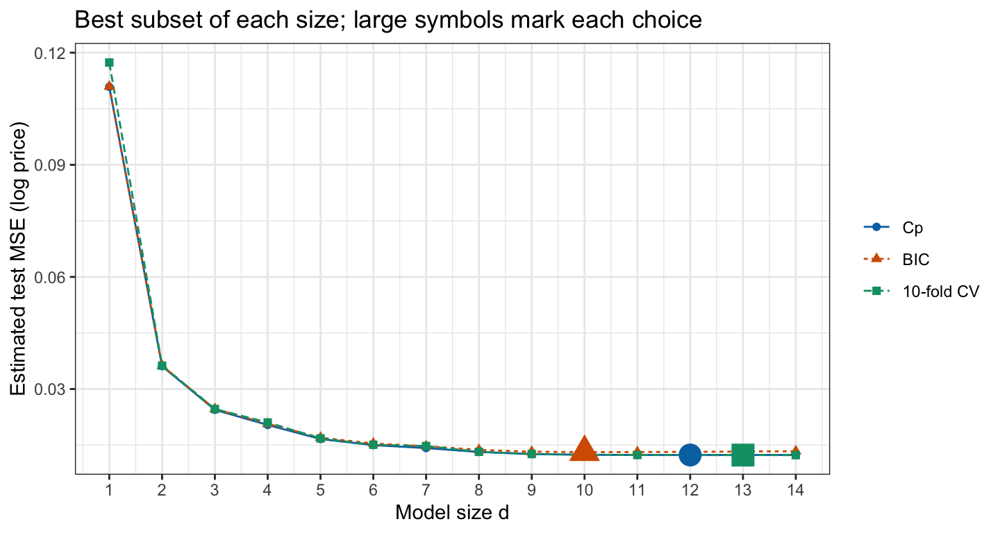
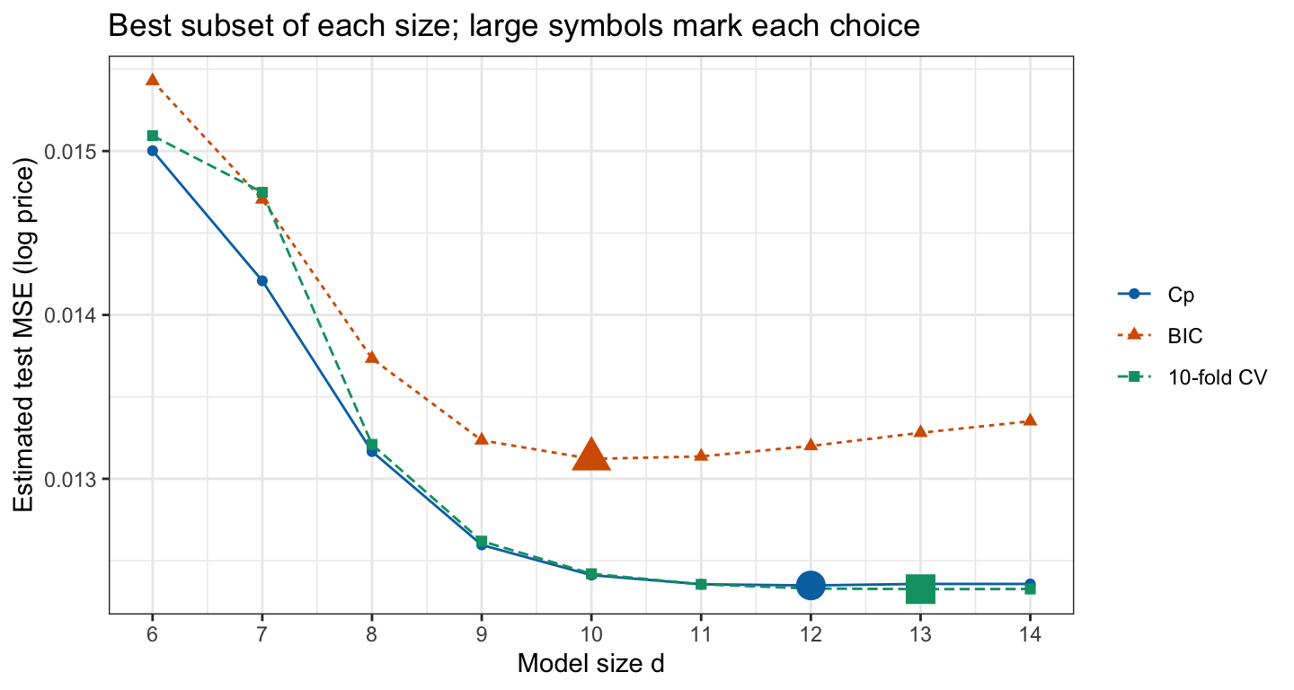
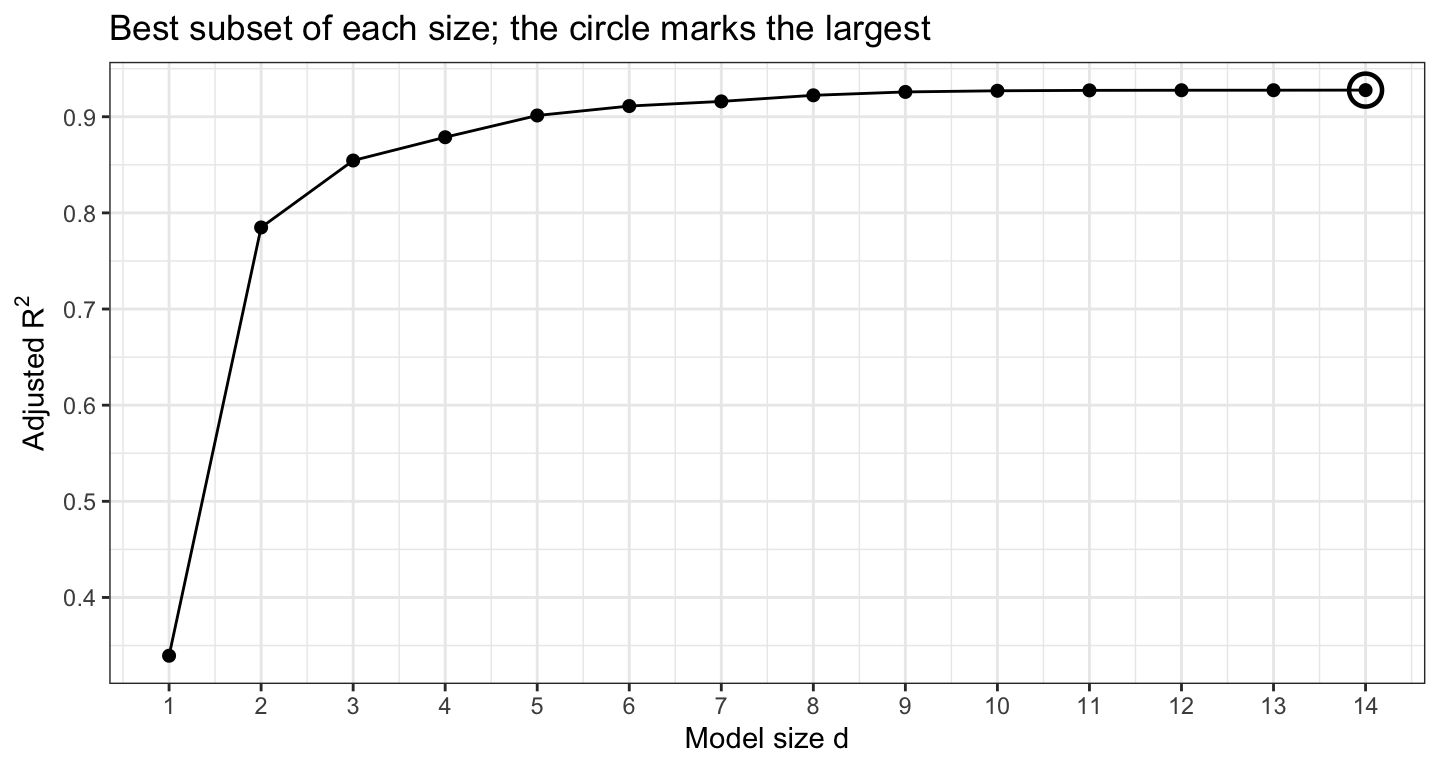
All four curves fall steeply over the first few sizes and then flatten: from $d = 10$ on, the cross-validation estimate is within 1% of its minimum. They disagree about where in the flat stretch to stop: the BIC chooses $d = 10$, $C_p$ $d = 12$, adjusted $R^2$ $d = 14$, and cross-validation $d = 13$. As the penalties predict, the BIC chooses the smallest model and adjusted $R^2$ the largest. $C_p$ and the cross-validation estimate are within 1% of each other at every size from $d = 8$ on, while the BIC, with its larger penalty, lies above both and rises after its minimum.

$C_p$ and cross-validation estimate different errors, although the figure plots both on one axis. $C_p$ estimates the error on new responses at the same feature values $x_i$ as these cars; cross-validation predicts held-out cars whose feature values the fit has not seen, which is the error on new cars. Below $d = 8$ the cross-validation estimate is the larger at every size, 0.1174 against 0.1109 for $C_p$ at $d = 1$, a gap that reflects this difference.

The differences in the flat stretch are small: the cross-validation estimate at the BIC’s size is only 0.8% above its minimum. Over 20 further random partitions into folds, cross-validation chooses $d = 10$ once, $d = 11$ 6 times, $d = 12$ 5 times, and $d = 14$ 8 times, so the size it chooses depends on the partition. Cross-validation needs no $\hat\sigma^2$ and does not rely on normal, constant-variance errors, at the price of 10 best subset searches instead of one.

20.5 Selected model

20.5.1 Coefficients

The criteria leave sizes 10 through 14 nearly tied, so the smallest of them, the BIC’s $\mathcal{M}_{10}$, is interpreted here: it is easiest to explain and its cross-validation estimate is within 0.8% of the smallest.

Code

selected_features <- features_of(best_which, d_bic)
dropped <- setdiff(features, selected_features)
selected <- lm(reformulate(selected_features, "log_price"), data = cars)
b <- coef(selected)
# Percent change in median price per unit; Mileage per 10,000 miles.
unit <- if_else(names(b) == "Mileage", 10000, 1)
coef_table <- tibble(Feature = names(b), Estimate = b,
                     Change = if_else(names(b) == "(Intercept)", NA_real_,
                                      100 * (exp(unit * b) - 1))) |>
  mutate(Estimate = formatC(Estimate, format = "g", digits = 4),
         Change = if_else(is.na(Change), "", paste0(fmt(Change, 1), "%"))) |>
  knitr::kable(col.names = c("Feature", "$\\hat\\beta_j$", "Change in median price"),
               align = "lrr",
               caption = paste("Change in median price per 10,000 miles for Mileage,",
                               "per cylinder for Cylinder, and from 0 to 1 for each",
                               "indicator."))
dropped_makes <- intersect(dropped, make_names)
kept_makes <- intersect(selected_features, make_names)
four_cyl_price <- exp(b[["(Intercept)"]] + 4 * b[["Cylinder"]])

Change in median price per 10,000 miles for Mileage, per cylinder for Cylinder, and from 0 to 1 for each indicator.
Feature	$\hat\beta_j$	Change in median price
(Intercept)	9.015
Mileage	-8.199e-06	-7.9%
Cylinder	0.1865	20.5%
Leather	0.03446	3.5%
Buick	0.1204	12.8%
Cadillac	0.4288	53.5%
Saab	0.7032	102.0%
convertible	0.1572	17.0%
coupe	-0.1178	-11.1%
hatchback	-0.2924	-25.4%
sedan	-0.1681	-15.5%

The model drops Cruise, Sound, Chevy, and Pontiac. With a normal error on the log scale, $e^{x_i\beta}$ is the median price, so $e^{\hat\beta_j}$ multiplies the median price per unit of feature $j$, a change of $100\left(e^{\hat\beta_j} - 1\right)\%$.

Intercept. $e^{\hat\beta_0}$ = $8,225 is the estimated median price when every feature is zero: no miles, no leather, a wagon, a reference make, and zero cylinders. No car has zero cylinders, so $\hat\beta_0$ only sets the level; the same car with four cylinders has estimated median price $e^{\hat\beta_0 + 4\hat\beta_{\texttt{Cylinder}}}$ = $17,341.
Reference make. Because Chevy and Pontiac were dropped, their cars share the intercept with Saturn: the reference make is now Chevy, Pontiac, and Saturn together, and each retained make coefficient (Buick, Cadillac, and Saab) compares that make with those three. Dropping a dummy variable merges its level into the reference.
Mileage. Each additional 10,000 miles multiplies the median price by $e^{10000\,\hat\beta_{\texttt{Mileage}}} = 0.921$, holding the other features fixed.
Other features. Each additional pair of cylinders multiplies the median price by $e^{2\hat\beta_{\texttt{Cylinder}}} = 1.452$, and the body style coefficients compare each style with a wagon.

20.5.2 Optimistic inference

summary(selected) reports standard errors and $p$-values as though these 10 features had been chosen before seeing the data. They were chosen because they fit these cars well, which makes both optimistic for two reasons.

Error variance. The standard errors are proportional to the selected model’s $\hat\sigma$, which comes from $RSS_d$, the smallest of 1,001 residual sums of squares of size $d = 10$. The smallest of many RSS values tends to be lower than the RSS of a model fixed in advance, so $\hat\sigma$ tends to be too small. On the cars the selected model has $\hat\sigma = 0.1108$ against 0.1103 for the largest model: with 804 cars the search lowers $\hat\sigma$ only a little, and dropping Cruise, Sound, Chevy, and Pontiac raises it by more.
Large $|t|$. A feature enters because its estimated coefficient is large relative to its standard error in these data, so its $|t|$ statistic is large and its $p$-value small, whatever its true coefficient.

The simulation below keeps the features of the 804 cars but replaces log price with independent normal noise with standard deviation 0.1103, so every true coefficient is zero. Each noise data set goes through best subset selection with the size chosen by $C_p$, and the selected model is refit with lm().

Code

n_noise <- 500
noise_sims <- map(seq_len(n_noise), \(r) {
  noise_cars <- mutate(cars, log_price = rnorm(n, 0, sigma(full_log)))
  s <- summary(regsubsets(log_price ~ ., data = noise_cars, nvmax = p))
  s2 <- sigma(lm(log_price ~ ., data = noise_cars))^2
  noise_tss <- sum((noise_cars$log_price - mean(noise_cars$log_price))^2)
  # Cp of sizes 0 to p; size 0 is the null model.
  d <- which.min((c(noise_tss, s$rss) + 2 * (0:p) * s2) / n) - 1
  kept <- if (d == 0) character(0) else colnames(s$which)[s$which[d, ]][-1]
  fit <- lm(reformulate(if (d == 0) "1" else kept, "log_price"), data = noise_cars)
  list(d = d, sigma2 = sigma(fit)^2,
       p_value = summary(fit)$coefficients[-1, "Pr(>|t|)"])
})
noise_any <- mean(map_dbl(noise_sims, "d") > 0)
noise_p <- unlist(map(noise_sims, "p_value"))
noise_small_p <- mean(noise_p < 0.05)
noise_sigma2_bias <- mean(map_dbl(noise_sims, "sigma2")) / sigma(full_log)^2 - 1
noise_plot <- ggplot(tibble(p_value = noise_p), aes(x = p_value)) +
  geom_histogram(aes(y = after_stat(density)), binwidth = 0.05, boundary = 0,
                 fill = "grey70", color = "grey30") +
  geom_hline(yintercept = 1, linetype = "dashed") +
  scale_x_continuous(limits = c(0, 1)) +
  labs(x = "p-value of a kept noise feature", y = "Density",
       title = paste(length(noise_p), "noise features kept by Cp in",
                     n_noise, "noise data sets"),
       caption = "Dashed line: the p-value of a feature chosen in advance is uniform.")

The histogram shows the $p$-values that summary() reports for every noise feature kept.

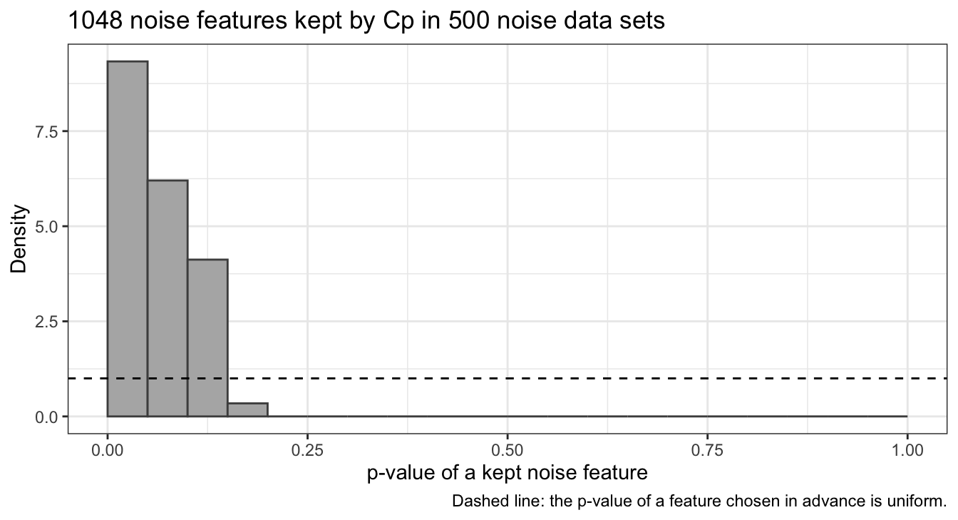
$C_p$ keeps at least one noise feature in 89.8% of the 500 data sets. The $p$-value of a feature chosen in advance is uniformly distributed, below 0.05 in 5% of data sets; 46.7% of the kept noise features have $p < 0.05$. The selected models’ $\hat\sigma^2$ averages 1.0% below $\sigma^2$, the first reason at work, and small here because $n$ is large relative to $p$.

20.6 Conclusion

Subset selection chooses which of $p$ candidate features a least squares model uses. Best subset selection fits every subset, $2^p$ models, keeps the one with the smallest RSS at each size $d$, and then chooses among sizes. Forward and backward stepwise selection build a nested path by adding or removing one feature at a time, fitting $1 + p(p+1)/2$ models; they are greedy, so their model of a given size need not be the best one, and backward selection requires $n > p$.

Within one size, the training RSS is a fair way to compare models. Across sizes it is not: the RSS and $R^2$ always improve as features are added, so they always choose the largest model. The training RSS underestimates the error on new responses at the same feature values by $2(d+1)\sigma^2$ on average, which $C_p$ (equivalent to AIC for Gaussian least squares) adds back, up to a constant. The BIC charges $\log(n)$ per feature instead of 2 and favors smaller models; adjusted $R^2$ charges least. Cross-validation estimates the error on new observations, at new feature values, directly, and because choosing the best model of each size is part of the fit, that search must be repeated inside every fold from the training folds only. Criteria and cross-validation often disagree where the estimated error is flat.

A selected model is interpreted like any regression, with one addition: dropping some dummy variables of a categorical explanatory variable merges those levels into the reference. Its standard errors and $p$-values ignore the selection and are optimistic: its $\hat\sigma$ comes from the smallest of many RSS values, and its features were kept because their $|t|$ statistics were large.

The next lecture, ridge regression, keeps all $p$ features and instead shrinks their coefficients toward zero by penalizing their size, with the amount of shrinkage chosen by cross-validation.