22  The Lasso

Slides for this lecture

TipLearning objectives

After this lecture you should be able to

• write the lasso criterion \(RSS + \lambda\sum_{j=1}^p\left|\beta_j\right|\) and its constrained form, contrast them with ridge regression’s, and state the fits as \(\lambda \to 0\) and for \(\lambda \ge \lambda_{\max}\),
• explain, using the constraint regions \(\sum_j\left|\beta_j\right| \le s\) and \(\sum_j\beta_j^2 \le s\) drawn over the RSS contours, why some lasso estimates are exactly zero and ridge estimates, except by coincidence, are not,
• derive the lasso estimate for orthogonal standardized features as soft thresholding of the least squares estimate, and compare it with ridge regression’s proportional shrinkage,
• read a lasso estimate path: which features enter first, and how many estimates are nonzero at each \(\lambda\),
• choose \(\lambda\) by \(k\)-fold cross-validation on the training data, evaluate the chosen model once on test data, and compare the lasso, ridge regression, and least squares by test MSE and by the features they keep, and
• explain, from repeated training samples, why the set of features the lasso selects is unstable and why the lasso estimator of a nonzero coefficient is biased toward zero, and explain why lm()’s standard errors and \(p\)-values do not apply to the lasso estimates.

22.1 Delivery times

22.1.1 Data

Question. Does a model that keeps only some of the 35 features predict delivery times better than one that uses all of them?

Data. The modeldata::deliveries orders of the Ridge Regression lecture: the delivery time time_to_delivery, in minutes, with hour, day, distance, and the counts item_01, …, item_27 of each menu item.

# The orders, and the two training sample sizes.
deliveries <- modeldata::deliveries
n_orders <- nrow(deliveries)
n_train <- 100
n_large <- 300

# Split the orders into training and test orders.
train_id <- sample(n_orders, n_train)
train <- deliveries[train_id, ]
test <- deliveries[-train_id, ]
n_test <- nrow(test)

# Folds for 10-fold cross-validation of the training orders.
n_folds <- 10
fold_labels <- rep(seq_len(n_folds), length.out = n_train)
fold_id <- sample(fold_labels)

These are the first random draws after the ridge lecture’s set.seed(20261017), so the split and the folds are the ridge lecture’s: 100 training orders and 9,912 test orders, set aside until the chosen model is evaluated. As there, the training sample is deliberately small relative to the 36 coefficients of the model, so that their estimates are poorly determined; the repeated samples at the end also use 300 training orders. The figure plots, for each item, the delivery times of the training orders that contain it.

NoteCode

# Number of training orders containing each item, and the median time.
item_names <- sprintf("item_%02d", 1:27)
orders_with <- colSums(train[item_names] > 0)
time_median <- median(train$time_to_delivery)

# One row per training order and item it contains, item_01 at the top.
item_levels <- rev(item_names)
item_long <- train |>
  pivot_longer(all_of(item_names),
               names_to = "item",
               values_to = "count") |>
  filter(count > 0) |>
  mutate(item = factor(item, levels = item_levels))
item_medians <- tapply(item_long$time_to_delivery, item_long$item, median)

# Delivery times by item, with the median for each item.
item_labels <- paste0(rev(item_names), " (", rev(orders_with), ")")
item_plot <- ggplot(item_long, aes(x = time_to_delivery, y = item)) +
  geom_vline(xintercept = time_median,
             linetype = "dashed",
             color = "grey50") +
  geom_point(position = position_jitter(width = 0, height = 0.15, seed = 1),
             size = 0.9,
             alpha = 0.6) +
  stat_summary(fun = median,
               fun.min = median,
               fun.max = median,
               geom = "crossbar",
               width = 0.7,
               color = "#D55E00") +
  scale_y_discrete(labels = item_labels) +
  labs(x = "Delivery time (minutes)",
       y = "Item (number of training orders containing it)",
       title = paste(n_train, "training orders"),
       caption = paste("Bars = median for orders with the item;",
                       "dashed line = median of all training orders."))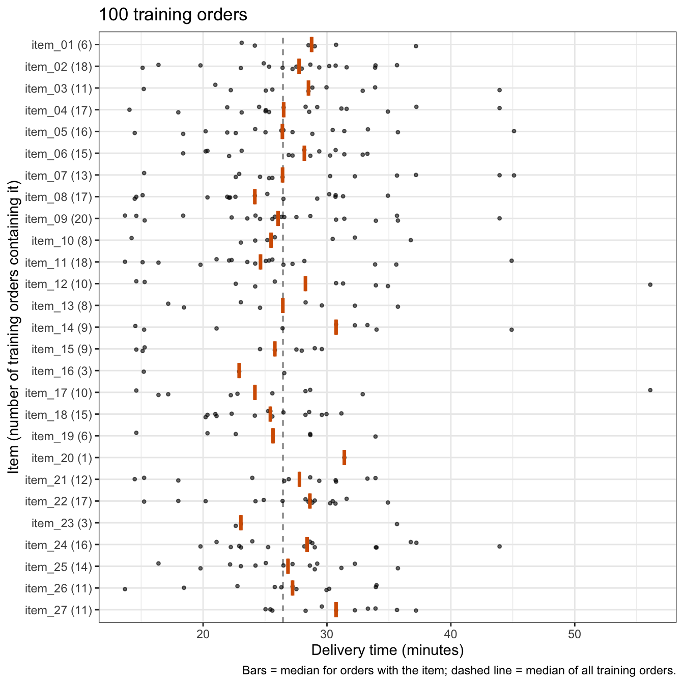

Each item appears in between 1 and 20 of the 100 training orders. The median delivery time of the orders containing an item ranges from 22.9 to 31.4 minutes, around the overall median of 26.5, and the times of the orders containing any one item vary widely. These orders also differ in distance, hour, and day, which the ridge lecture showed matter, so a difference between items here need not be an effect of the items.

22.1.2 Ridge estimates

# Model matrix of the features, without the column of ones.
model_matrix <- function(data) {
  X <- model.matrix(time_to_delivery ~ ., data = data)
  X[, -1]
}

# Features and responses of the training and test orders.
X_train <- model_matrix(train)
y_train <- train$time_to_delivery
X_test <- model_matrix(test)
y_test <- test$time_to_delivery
p <- ncol(X_train)

# Mean squared error.
mse <- function(y, y_hat) {
  mean((y - y_hat)^2)
}

# Standard deviation with divisor n.
sd_n <- function(v) {
  deviations <- v - mean(v)
  sqrt(mean(deviations^2))
}

# Standard deviations of the training responses and of each feature.
s_y <- sd_n(y_train)
x_scale <- apply(X_train, 2, sd_n)

As in the ridge lecture, day enters as 6 dummy variables with Monday as the reference, so there are \(p = 35\) features. The figure repeats that lecture’s estimate path: the ridge estimate of each standardized coefficient, fit to the training orders, against \(\lambda\).

NoteCode

# Grid of lambda values, and the ridge lecture's conversion of lambda to
# glmnet()'s scale.
lambda_grid <- 10^seq(3, -2, length.out = 101)
to_glmnet_ridge <- function(lambda) {
  lambda * s_y / n_train
}

# Feature groups for the legend.
day_group <- paste0("day (", nlevels(train$day) - 1, " dummies)")
item_group <- paste0("items (", length(item_names), ")")
group_levels <- c("distance", "hour", day_group, item_group)

# The group of each feature name.
feature_group <- function(feature) {
  is_numeric <- feature %in% c("distance", "hour")
  is_day <- str_starts(feature, "day")
  case_when(is_numeric ~ feature,
            is_day ~ day_group,
            TRUE ~ item_group)
}

# Standardized estimates of a glmnet() path, one row per feature and lambda.
path_data <- function(fit, lambdas) {
  stopifnot(length(fit$lambda) == length(lambdas))
  b <- as.matrix(coef(fit))[-1, ] * x_scale
  as_tibble(b, rownames = "feature") |>
    pivot_longer(-feature, values_to = "estimate") |>
    mutate(lambda = rep(lambdas, times = p),
           group = feature_group(feature),
           group = factor(group, levels = group_levels))
}

# Standardized estimates against lambda, one line per feature.
path_plot <- function(path, title) {
  ggplot(path,
         aes(x = lambda,
             y = estimate,
             group = feature,
             color = group,
             linetype = group)) +
    geom_hline(yintercept = 0, color = "grey50") +
    geom_line() +
    log_lambda +
    scale_color_manual(values = okabe_ito[c(4, 5, 3, 1)]) +
    scale_linetype_manual(values = c("solid", "longdash", "dotdash",
                                     "dotted")) +
    labs(x = expression(lambda ~ "(log scale)"),
         y = "Standardized estimate\n(minutes per standard deviation)",
         color = NULL,
         linetype = NULL,
         title = title) +
    theme(legend.position = "bottom")
}

# Ridge path fit to the training orders.
ridge_path_fit <- glmnet(X_train,
                         y_train,
                         alpha = 0,
                         lambda = to_glmnet_ridge(lambda_grid),
                         thresh = 1e-12)
ridge_path_data <- path_data(ridge_path_fit, lambda_grid)
ridge_title <- paste("Ridge estimate path,", n_train, "training orders")
ridge_path_plot <- path_plot(ridge_path_data, ridge_title)

# Fewest nonzero ridge estimates at any lambda on the grid.
ridge_estimates <- as.matrix(coef(ridge_path_fit))[-1, ]
ridge_min_nonzero <- min(colSums(ridge_estimates != 0))

# The item estimate closest to zero at the largest lambda.
ridge_smallest <- ridge_path_data |>
  filter(lambda == max(lambda_grid), str_starts(feature, "item")) |>
  slice_min(abs(estimate), n = 1)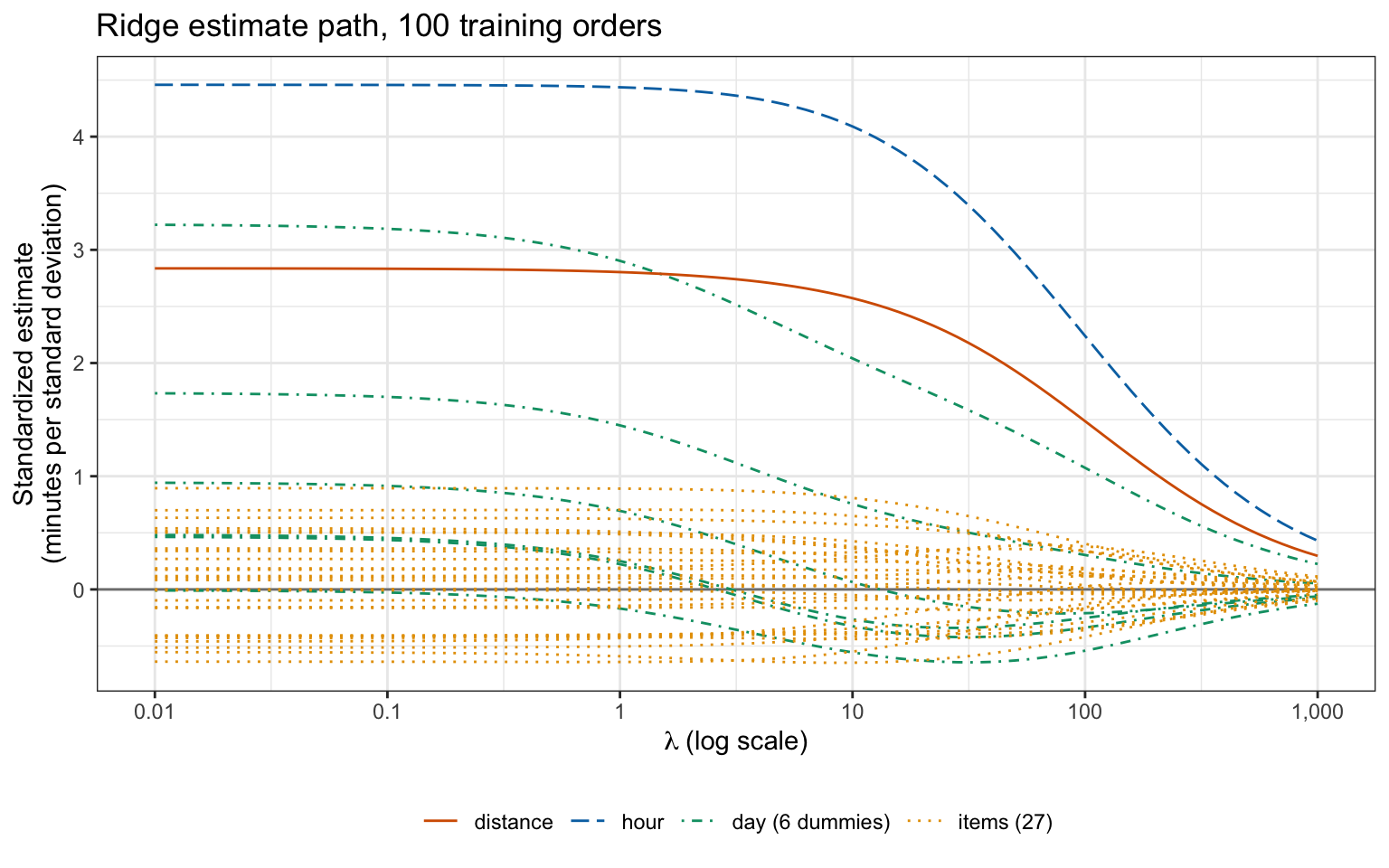

The ridge estimates shrink toward zero as \(\lambda\) grows, but at every one of the 101 values of \(\lambda\) on the grid all 35 are nonzero. At \(\lambda = 1{,}000\) the item estimate closest to zero, that of item_23, is still \(4.0 \times 10^{-3}\) minutes per standard deviation.

22.2 Lasso

The geometry of this section uses two features: the standardized distance and hour of the training orders. The figure plots the delivery time against each.

NoteCode

# Standardize distance and hour with the training means and standard
# deviations.
two_names <- c("distance", "hour")
X_two <- X_train[, two_names]
X_two_centered <- sweep(X_two, 2, colMeans(X_two))
Z2 <- sweep(X_two_centered, 2, x_scale[two_names], "/")

# Delivery time against each standardized feature.
two_long <- as_tibble(Z2) |>
  mutate(time = y_train) |>
  pivot_longer(-time, names_to = "feature")
two_plot <- ggplot(two_long, aes(x = value, y = time)) +
  geom_point(size = 1) +
  facet_wrap(~ paste("Standardized", feature)) +
  labs(x = "Standard deviations from the training mean",
       y = "Delivery time (minutes)",
       title = paste(n_train, "training orders"))

# Correlation of the two standardized features.
two_cor <- cor(Z2)[1, 2]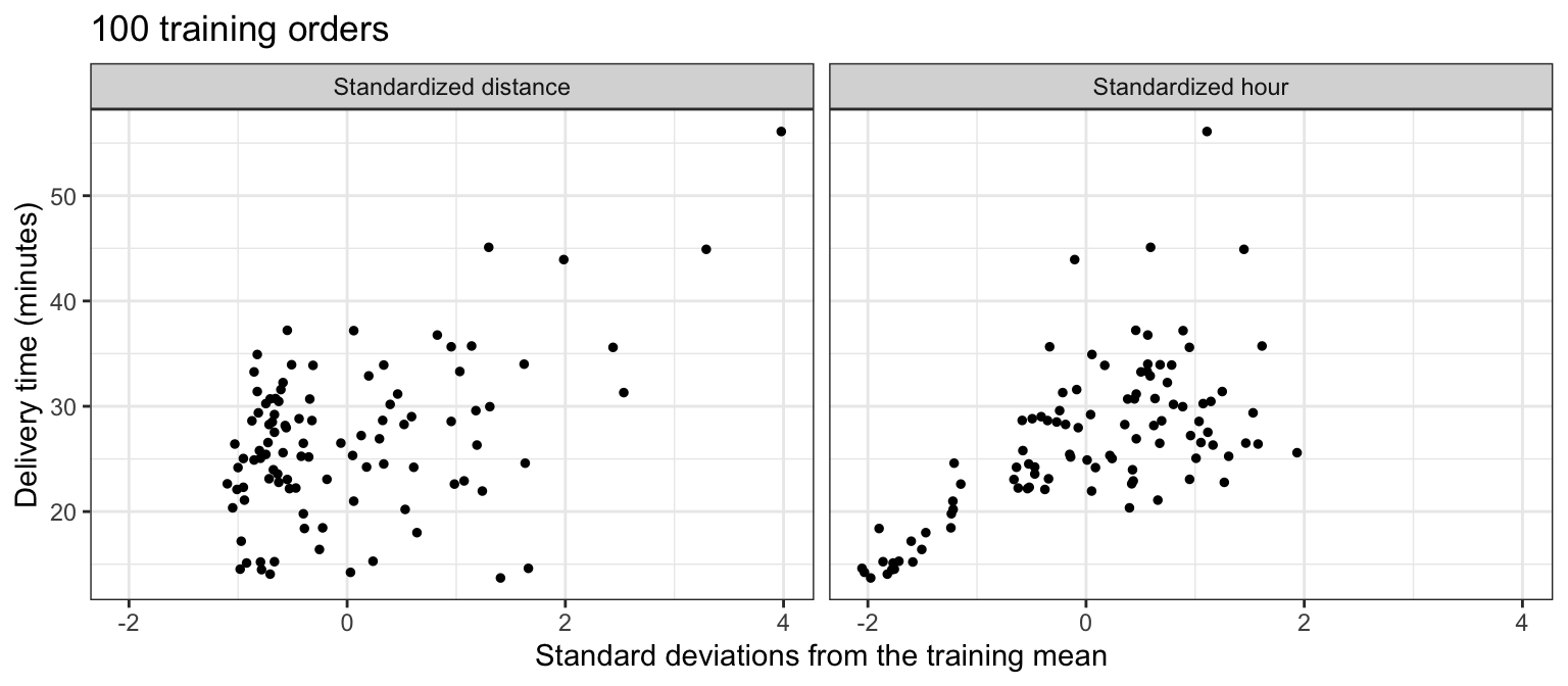

Delivery time rises with both, and the two are nearly uncorrelated in the training orders (correlation 0.06).

22.2.1 Penalized criterion

The lasso estimates the coefficients by minimizing

\[\sum_{i=1}^n\left(y_i - \beta_0 - \sum_{j=1}^p\beta_j\tilde x_{ij}\right)^2 + \lambda\sum_{j=1}^p\left|\beta_j\right| = RSS + \lambda\sum_{j=1}^p\left|\beta_j\right|,\]

where

• \(y_i\) is the delivery time of training order \(i = 1, \ldots, n\), with \(n = 100\),
• \(\tilde x_{ij} = \left(x_{ij} - \bar x_j\right)/s_j\) is feature \(j\) of order \(i\) standardized, with \(\bar x_j\) the mean of feature \(j\) over the \(n\) training orders and \(s_j\) its standard deviation, computed with divisor \(n\),
• \(\beta_0\) and \(\beta_1, \ldots, \beta_p\) are the coefficients on the standardized scale, where \(\beta_j\) is \(s_j\) times the coefficient of feature \(j\) on the original scale, as in the Ridge Regression lecture,
• \(\lambda \ge 0\) is the tuning parameter, and
• \(\lambda\sum_{j=1}^p\left|\beta_j\right|\) is the \(\ell_1\) penalty, in place of ridge regression’s \(\ell_2\) penalty \(\lambda\sum_{j=1}^p\beta_j^2\).

The intercept is not penalized and the features are standardized, for the reasons the ridge lecture gave; the \(\ell_1\) penalty is no more scale equivariant than the \(\ell_2\) penalty. The criterion is convex but not differentiable where some \(\beta_j = 0\), and in general its minimum has no closed form.

At \(\lambda = 0\) the lasso is least squares. Unlike ridge regression, it reaches the null model at a finite \(\lambda\). The standardized features are centered, so whatever the slopes, the intercept that minimizes the criterion is \(\hat\beta_0 = \bar y\), the mean delivery time of the training orders; take \(\beta_0 = \bar y\). At \(\beta = 0\), changing one coefficient \(\beta_j\) to \(t\) then changes the RSS by \(-2t\sum_i\tilde x_{ij}\left(y_i - \bar y\right) + nt^2\) and the penalty by \(\lambda\left|t\right|\), so no estimate can leave zero when

\[\lambda \ge \lambda_{\max} = \max_{j}\, 2\left|\sum_{i=1}^n\tilde x_{ij}\left(y_i - \bar y\right)\right|,\]

and, because the criterion is convex and the penalty is a sum over \(j\), every slope estimate is zero and every prediction is \(\hat\beta_0 = \bar y\), the null model.

# Standardized training features.
X_centered <- sweep(X_train, 2, colMeans(X_train))
X_std <- sweep(X_centered, 2, x_scale, "/")

# Twice the absolute sum of each standardized feature times the centered
# responses; the largest is lambda_max.
y_centered <- y_train - mean(y_train)
feature_sums <- drop(crossprod(X_std, y_centered))
lambda_scores <- 2 * abs(feature_sums)
lambda_max <- max(lambda_scores)

For the training orders \(\lambda_{\max} = 967.4\), set by hour, the feature most correlated with the delivery time.

22.2.2 Constraint regions

Minimizing the lasso criterion is equivalent to minimizing the RSS subject to

\[\sum_{j=1}^p\left|\beta_j\right| \le s, \qquad\text{and for ridge regression}\qquad \sum_{j=1}^p\beta_j^2 \le s,\]

where \(s \ge 0\) is a budget: each \(\lambda\) corresponds to some \(s\), a smaller \(\lambda\) to a larger \(s\). The budget \(s\) is the textbook’s symbol; it is unrelated to the standard deviations \(s_j\) above and \(s_y\) below. For the two standardized features above, the region is a diamond for the lasso and a disk for ridge regression, and the RSS has elliptical contours centered at the least squares estimate. The constrained estimate is where the smallest contour touches the region.

NoteCode

# Least squares estimate for the two standardized features; the RSS is a
# quadratic in (b1, b2) centered there.
A2 <- crossprod(Z2)
Z2_y <- crossprod(Z2, y_centered)
b_two <- drop(solve(A2, Z2_y))
rss_min <- sum((y_centered - Z2 %*% b_two)^2)
rss_two <- function(b1, b2) {
  d1 <- b1 - b_two[1]
  d2 <- b2 - b_two[2]
  rss_min + A2[1, 1] * d1^2 + 2 * A2[1, 2] * d1 * d2 + A2[2, 2] * d2^2
}

# While only the first feature to enter is nonzero, the lasso keeps the other
# at zero; that holds for every budget below s_enter.
a <- drop(Z2_y) / n_train
first <- which.max(abs(a))
sign_product <- sign(a[first]) * sign(a[-first])
s_enter <- (abs(a[first]) - abs(a[-first])) / (1 - two_cor * sign_product)

# The budget drawn. The prose writes the corner as (0, s): hour enters first.
s_budget <- 1.5
stopifnot(s_budget < s_enter, first == 2)

# Lasso estimate at this budget: the corner on the first feature's axis.
b_lasso2 <- replace(c(0, 0), first, sign(a[first]) * s_budget)

# Ridge estimate with sum of squares s_budget^2, on the disk through the
# diamond's corners: solve for the lambda that puts it there.
ridge2 <- function(l) {
  lhs <- A2 + l * diag(2)
  drop(solve(lhs, Z2_y))
}
ridge2_excess <- function(l) {
  b <- ridge2(l)
  sqrt(sum(b^2)) - s_budget
}
l_budget <- uniroot(ridge2_excess, c(0, 1e5))$root
b_ridge2 <- ridge2(l_budget)

# Grid of (b1, b2) values for the RSS contours.
grid <- expand_grid(b1 = seq(-2, 5, length.out = 281),
                    b2 = seq(-2, 6, length.out = 321)) |>
  mutate(rss = rss_two(b1, b2))

# The lasso region (a diamond) and the ridge region (a disk).
diamond <- tibble(b1 = c(s_budget, 0, -s_budget, 0),
                  b2 = c(0, s_budget, 0, -s_budget))
disk <- tibble(t = seq(0, 2 * pi, length.out = 361),
               b1 = s_budget * cos(t),
               b2 = s_budget * sin(t))

# RSS contours and the least squares estimate.
contour_breaks <- rss_two(b_two[1], b_two[2]) + 200 * (1:6)^2
geometry_title <- paste(n_train,
                        "training orders; grey ellipses = RSS contours")
geometry_base <- ggplot(grid, aes(x = b1, y = b2)) +
  geom_hline(yintercept = 0, color = "grey70") +
  geom_vline(xintercept = 0, color = "grey70") +
  geom_contour(aes(z = rss),
               breaks = contour_breaks,
               color = "grey60",
               linewidth = 0.3) +
  annotate("point",
           x = b_two[1],
           y = b_two[2],
           shape = 4,
           size = 3,
           stroke = 1.3) +
  annotate("text",
           x = b_two[1],
           y = b_two[2],
           label = "Least squares",
           vjust = -1,
           size = 3.5) +
  coord_equal(xlim = c(-2, 5), ylim = c(-2, 6)) +
  labs(x = expression(beta[1] ~ "(standardized distance)"),
       y = expression(beta[2] ~ "(standardized hour)"),
       title = geometry_title)

# Add a constraint region, the contour through its estimate, and the
# estimate.
add_region <- function(region, b, color, linetype, label) {
  geometry_base +
    geom_polygon(data = region,
                 fill = color,
                 alpha = 0.25,
                 color = color) +
    geom_contour(aes(z = rss),
                 breaks = rss_two(b[1], b[2]),
                 color = color,
                 linetype = linetype,
                 linewidth = 0.9) +
    annotate("point",
             x = b[1],
             y = b[2],
             shape = 16,
             size = 3,
             color = color) +
    labs(caption = label)
}

# Least squares estimates whose constrained estimate at this budget is the
# corner b_lasso2: b_lasso2 + mu * solve(A2) %*% g, mu >= 0, with g a normal
# to the region there. The diamond has normals g = (u, 1), |u| <= 1, a wedge;
# the disk has the single normal b_lasso2, a ray.
A2_inv <- solve(A2)
normal <- function(u) {
  replace(c(u, u), first, sign(a[first]))
}
unit <- function(v) {
  v / sqrt(sum(v^2))
}
far <- 50

# The wedge: the corner and a far point along each of its two edges.
normal_low <- normal(-1)
normal_high <- normal(1)
edge_low <- unit(drop(A2_inv %*% normal_low))
edge_high <- unit(drop(A2_inv %*% normal_high))
wedge_points <- rbind(b_lasso2,
                      b_lasso2 + far * edge_low,
                      b_lasso2 + far * edge_high)
wedge <- as_tibble(wedge_points, .name_repair = \(x) c("b1", "b2"))

# The ray, and its angle from the first feature's axis.
ray_direction <- unit(drop(A2_inv %*% b_lasso2))
ray_end <- b_lasso2 + far * ray_direction
ray_rise <- abs(ray_end[-first] - b_lasso2[-first])
ray_run <- abs(ray_end[first] - b_lasso2[first])
ray_angle <- atan2(ray_rise, ray_run)

# Where the least squares estimate lies in the wedge:
# A2 (b_two - corner) = mu * (u, 1) with |u| <= 1.
wedge_normal <- drop(A2 %*% (b_two - b_lasso2))
wedge_u <- wedge_normal[-first] / wedge_normal[first]

# The wedge and the ray at the corner.
corner_caption <- paste0(
  "Budget ", s_budget,
  ". Shaded: least squares estimates whose lasso estimate is the corner;\n",
  "dashed line: those whose ridge estimate is that point."
)
corner_plot <- geometry_base +
  geom_polygon(data = wedge, fill = okabe_ito[5], alpha = 0.25) +
  geom_polygon(data = diamond, fill = NA, color = okabe_ito[5]) +
  geom_path(data = disk, color = okabe_ito[4]) +
  annotate("segment",
           x = b_lasso2[1],
           y = b_lasso2[2],
           xend = ray_end[1],
           yend = ray_end[2],
           color = okabe_ito[4],
           linetype = "dashed",
           linewidth = 0.9) +
  annotate("point",
           x = b_lasso2[1],
           y = b_lasso2[2],
           shape = 16,
           size = 3) +
  labs(caption = corner_caption)

# The four tabs.
lasso_caption <- bquote("Lasso region" ~ abs(beta[1]) + abs(beta[2]) <=
                          .(s_budget) *
                          "; solid ellipse = contour through the estimate")
ridge_caption <- bquote("Ridge region" ~ beta[1]^2 + beta[2]^2 <=
                          .(s_budget)^2 *
                          "; dashed ellipse = contour through the estimate")
geometry_plots <- list(
  geometry_base,
  add_region(diamond, b_lasso2, okabe_ito[5], "solid", lasso_caption),
  add_region(disk, b_ridge2, okabe_ito[4], "dashed", ridge_caption),
  corner_plot
)

RSS contours

+ Lasso

+ Ridge

Estimates at the corner

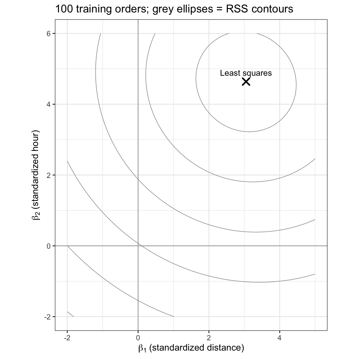
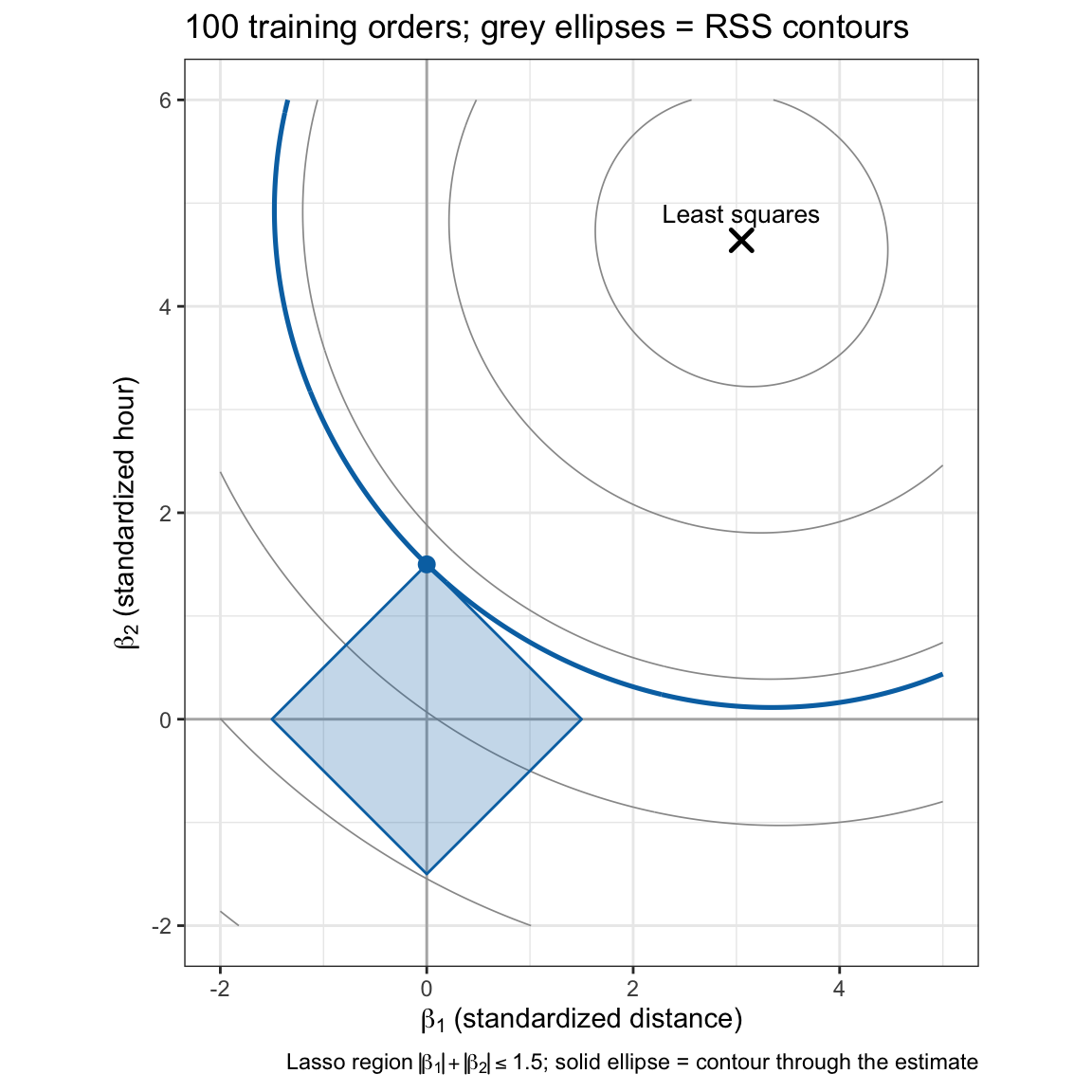
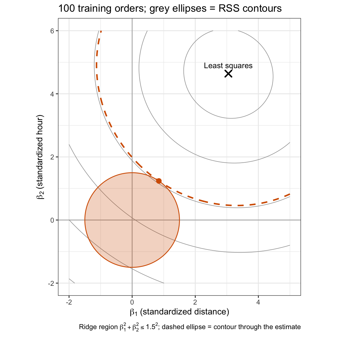
The least squares estimate, \(\left(3.05, 4.64\right)\), lies outside both regions, so each constrained estimate is on the boundary. With budget \(s = 1.5\) the smallest contour touches the diamond at its corner \(\left(0.00, 1.50\right)\): the estimate of the distance coefficient is exactly zero. The disk \(\beta_1^2 + \beta_2^2 \le 1.5^2\), through the same corners, is touched at \(\left(0.85, 1.24\right)\), where neither estimate is zero.

Which point of the boundary is touched depends on where the least squares estimate \(\hat\beta\) is. Write \(\mathbf{A} = \tilde{\mathbf{X}}^\top\tilde{\mathbf{X}}\), with \(\tilde{\mathbf{X}}\) here the \(n \times 2\) matrix of the two standardized features, so that the RSS is \(\left(\beta - \hat\beta\right)^\top\mathbf{A}\left(\beta - \hat\beta\right)\) plus a constant. At a constrained estimate \(b\) on the boundary, the direction in which the RSS decreases fastest, \(-2\mathbf{A}\left(b - \hat\beta\right)\), must be an outward normal \(g\) of the region at \(b\), or moving along the boundary would lower the RSS; so \(\hat\beta = b + \mu\mathbf{A}^{-1}g\) for some \(\mu \ge 0\).

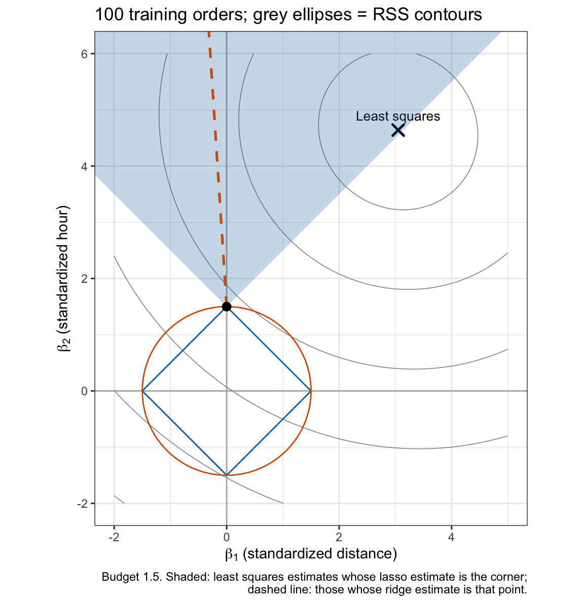
• On the disk of radius \(s\), through the diamond’s corners, the only outward normal at the axis point \((0, s)\) is \((0, 1)^\top\), so the least squares estimates whose ridge estimate is \((0, s)\) form a single ray from that point, in the direction \(\mathbf{A}^{-1}(0, 1)^\top\).
• At the diamond’s corner \((0, s)\) every \(g = (u, 1)^\top\) with \(\left|u\right| \le 1\) is an outward normal, so the least squares estimates whose lasso estimate is the corner fill a wedge.

The last tab draws both for \(s = 1.5\). The ray is tilted 3.7 degrees from the hour axis. With uncorrelated features \(\mathbf{A}\) would be \(n\mathbf{I}_2\) and the ray would run along the axis, so that only a least squares estimate on the axis would give a zero estimate. Either way the ray has no area, and a zero ridge estimate is a coincidence. The wedge has area, and the least squares estimate of the training orders falls inside it, near its edge (\(u = 0.97\)): the lasso keeps the distance estimate at zero for every budget below \(s = 1.59\).

The figure shows one budget and two nearly uncorrelated features; it illustrates the mechanism but does not show how often it acts. In \(p\) dimensions the region \(\sum_j\left|\beta_j\right| \le s\) has corners and edges on which many \(\beta_j\) are zero at once, and the least squares estimates whose lasso estimate lies on one of them fill a set of positive volume. For ridge regression the least squares estimates that give some ridge estimate exactly zero fill a set of zero volume.

Best subset selection is the same problem with the budget \(\sum_j\mathrm{I}\left(\beta_j \ne 0\right) \le s\) on the number of nonzero coefficients; that count, used as a penalty, is the \(\ell_0\) penalty. It is not convex, and minimizing it means searching over subsets. The lasso replaces it with a convex relaxation, the \(\ell_1\) budget, which can be minimized quickly.

22.2.3 Soft thresholding

Write \(\tilde{\mathbf{X}}\) now for the \(n \times p\) matrix of all \(p\) standardized features, without a column of ones. When they are orthogonal, \(\tilde{\mathbf{X}}^\top\tilde{\mathbf{X}} = n\mathbf{I}_p\) with \(\mathbf{I}_p\) the \(p \times p\) identity matrix, the least squares estimate is \(\hat\beta_j = \sum_i\tilde x_{ij}\left(y_i - \bar y\right)/n\), and

\[RSS = \sum_{i=1}^n\left(y_i - \bar y\right)^2 - 2n\sum_{j=1}^p\beta_j\hat\beta_j + n\sum_{j=1}^p\beta_j^2 = c + n\sum_{j=1}^p\left(\beta_j - \hat\beta_j\right)^2,\]

with \(\hat\beta_0 = \bar y\) and \(c\) not depending on \(\beta\). The lasso criterion splits into one problem per coefficient: minimize \(n\left(\beta_j - \hat\beta_j\right)^2 + \lambda\left|\beta_j\right|\).

• For \(\beta_j > 0\) the derivative \(2n\left(\beta_j - \hat\beta_j\right) + \lambda\) is zero at \(\beta_j = \hat\beta_j - \lambda/(2n)\), which is positive only if \(\hat\beta_j > \lambda/(2n)\).
• For \(\beta_j < 0\), likewise \(\beta_j = \hat\beta_j + \lambda/(2n)\), negative only if \(\hat\beta_j < -\lambda/(2n)\).
• Otherwise \(\left|\hat\beta_j\right| \le \lambda/(2n)\), the criterion decreases toward \(\beta_j = 0\) from both sides, and the minimum is \(\beta_j = 0\).

Together,

\[\hat\beta^L_{\lambda j} = \text{sign}\left(\hat\beta_j\right)\left(\left|\hat\beta_j\right| - \frac{\lambda}{2n}\right)_+, \qquad \hat\beta^R_{\lambda j} = \frac{n}{n + \lambda}\hat\beta_j,\]

where

• \(\hat\beta^L_{\lambda j}\) is the lasso estimate of standardized coefficient \(j\) for tuning parameter \(\lambda\), and \(\hat\beta^R_{\lambda j}\) the ridge estimate of the ridge lecture,
• \((u)_+ = \max(u, 0)\), and
• the map from \(\hat\beta_j\) to \(\hat\beta^L_{\lambda j}\) is soft thresholding at \(\lambda/(2n)\).

NoteCode

# Soft thresholding of b at t.
soft <- function(b, t) {
  sign(b) * pmax(abs(b) - t, 0)
}

# Orthogonalized features: sqrt(n) times an orthonormal basis for the span of
# the standardized training features, and their least squares estimates.
Z_orth <- sqrt(n_train) * qr.Q(qr(X_std))
b_orth <- drop(crossprod(Z_orth, y_centered)) / n_train

# The lasso at lambda = 150 by glmnet(), supplied lambda / (2n).
lambda_orth <- 150
orth_threshold <- lambda_orth / (2 * n_train)
orth_fit <- glmnet(Z_orth,
                   y_train,
                   alpha = 1,
                   lambda = orth_threshold,
                   thresh = 1e-14)
orth_lasso <- coef(orth_fit)[-1, 1]

# Largest difference between the glmnet() estimates and soft thresholding.
orth_soft <- soft(b_orth, orth_threshold)
orth_diff <- max(abs(orth_lasso - orth_soft))

# The same fit with the s_y of ridge regression's conversion carried over.
orth_wrong_fit <- glmnet(Z_orth,
                         y_train,
                         alpha = 1,
                         lambda = s_y * orth_threshold,
                         thresh = 1e-14)
orth_wrong <- coef(orth_wrong_fit)[-1, 1]

# Least squares, ridge, and lasso estimates as functions of the least squares
# estimate.
rule_labels <- c("Least squares", "Ridge", "Lasso")
b_range <- seq(-1.1, 1.1, length.out = 401) * max(abs(b_orth))
rules <- tibble(b = b_range) |>
  mutate(`Least squares` = b,
         Ridge = n_train / (n_train + lambda_orth) * b,
         Lasso = soft(b, lambda_orth / (2 * n_train))) |>
  pivot_longer(-b, names_to = "rule", values_to = "estimate") |>
  mutate(rule = factor(rule, levels = rule_labels))

# The rules as lines, the glmnet() estimates as circles.
orth_points <- tibble(b = b_orth, estimate = orth_lasso)
soft_title <- bquote(lambda == .(lambda_orth) * ", n =" ~ .(n_train))
soft_plot <- ggplot(rules, aes(x = b, y = estimate)) +
  geom_line(aes(color = rule, linetype = rule), linewidth = 0.9) +
  geom_point(data = orth_points, shape = 1, size = 2) +
  scale_color_manual(values = okabe_ito[c(1, 4, 5)]) +
  scale_linetype_manual(values = c("dotted", "dashed", "solid")) +
  coord_equal() +
  labs(x = "Least squares estimate (orthogonalized feature)",
       y = "Estimate",
       color = NULL,
       linetype = NULL,
       title = soft_title,
       caption = paste("Circles: glmnet() lasso estimates for the",
                       "orthogonalized training features.")) +
  theme(legend.position = "bottom")

The delivery features are not orthogonal, so the figure uses orthogonalized versions: \(\sqrt{n}\) times an orthonormal basis for the span of the standardized training features, 35 centered columns with \(\tilde{\mathbf{X}}^\top\tilde{\mathbf{X}} = n\mathbf{I}_p\) exactly and no meaning of their own. The lines are the formulas at \(\lambda = 150\); the circles are the lasso estimates glmnet() computes for these features, with \(\lambda\) converted as in the next subsection.

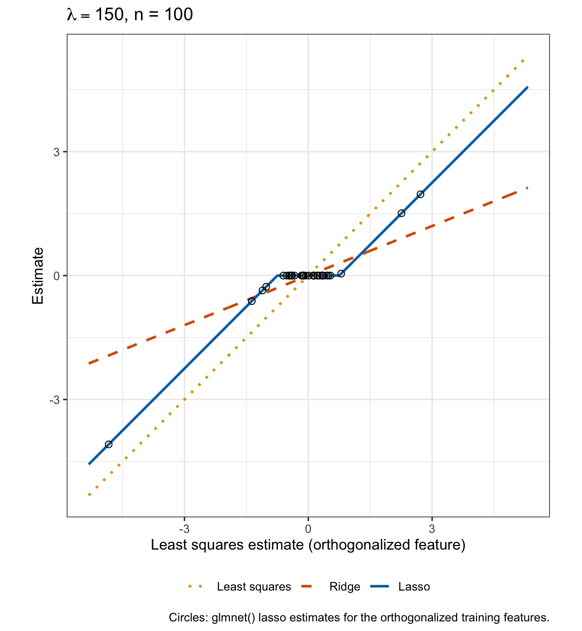
At \(\lambda = 150\) the ridge factor \(n/(n + \lambda)\) is 0.40. Ridge regression multiplies every estimate by that factor, so it moves the large estimates furthest. The lasso threshold \(\lambda/(2n)\) is 0.75, in the units of the estimates. The lasso moves every estimate larger than 0.75 in absolute value toward zero by exactly that amount, and sets the other 28 of the 35 to zero, moving each of them by its own magnitude. The glmnet() estimates match soft thresholding to within \(1.4 \times 10^{-15}\).

22.2.4 glmnet scaling

glmnet::glmnet() with alpha = 1 fits the lasso, with documented criterion

\[\frac{1}{2n}RSS + \lambda_{\text{glmnet}}\sum_{j=1}^p\left|\beta_j\right|,\]

or, multiplied by \(2n\), \(RSS + 2n\lambda_{\text{glmnet}}\sum_j\left|\beta_j\right|\). As the ridge lecture explained, glmnet() also divides \(y\) and the supplied \(\lambda_{\text{glmnet}}\) by \(s_y\), the standard deviation of the responses \(y_1, \ldots, y_n\) computed with divisor \(n\). Fitting \(y/s_y\) with coefficients \(\beta/s_y\) and tuning parameter \(\lambda_{\text{glmnet}}/s_y\) divides both the RSS and the penalty \(2n\left(\lambda_{\text{glmnet}}/s_y\right)\sum_j\left|\beta_j/s_y\right|\) by \(s_y^2\), which leaves the minimizer unchanged. For the lasso the two divisions cancel:

\[\lambda = 2n\,\lambda_{\text{glmnet}},\]

with no \(s_y\), unlike ridge regression’s \(\lambda = n\lambda_{\text{glmnet}}/s_y\). The circles in the soft-thresholding figure were computed at \(\lambda_{\text{glmnet}} = 150 / (2 \cdot 100) = 0.75\) and fall on the formula, which checks the conversion. The \(s_y\) of ridge regression’s conversion must not be carried over: the analogous \(\lambda = 2n\lambda_{\text{glmnet}}/s_y\) would supply \(\lambda_{\text{glmnet}} = 5.51\), \(s_y = 7.35\) times as large, and glmnet() would then set all 35 estimates to zero, against the 28 of soft thresholding at \(\lambda = 150\).

# This chapter's lambda to glmnet()'s, for a fit to n orders.
to_glmnet <- function(lambda, n = n_train) {
  lambda / (2 * n)
}

# glmnet()'s lambda to this chapter's.
to_chapter <- function(lambda_glmnet, n = n_train) {
  2 * n * lambda_glmnet
}

glmnet() minimizes the criterion by coordinate descent: it cycles through the coefficients, minimizing over one at a time with the others fixed. With the others fixed, the problem in \(\beta_j\) is the one-coefficient problem above, with \(\hat\beta_j\) replaced by the least squares estimate from regressing the partial residuals \(y_i - \bar y - \sum_{j' \ne j}\beta_{j'}\tilde x_{ij'}\) on \(\tilde x_{ij}\), so each step is a soft thresholding. From here on \(\lambda\) is this chapter’s, converted where glmnet() is used.

22.3 Estimate path

NoteCode

# Lasso path fit to the training orders.
lasso_grid <- 10^seq(3, -1, length.out = 81)
lasso_path_fit <- glmnet(X_train,
                         y_train,
                         alpha = 1,
                         lambda = to_glmnet(lasso_grid),
                         thresh = 1e-12)
lasso_path_data <- path_data(lasso_path_fit, lasso_grid)
lasso_title <- paste("Lasso estimate path,", n_train, "training orders")
lasso_path_plot <- path_plot(lasso_path_data, lasso_title)

# Number of nonzero estimates against lambda, lasso and ridge regression.
ridge_lasso <- c("Ridge", "Lasso")
nonzero_counts <- tibble(lambda = lasso_grid,
                         Lasso = lasso_path_fit$df,
                         Ridge = p) |>
  pivot_longer(-lambda, names_to = "method", values_to = "n") |>
  mutate(method = factor(method, levels = ridge_lasso))
nonzero_plot <- ggplot(nonzero_counts,
                       aes(x = lambda,
                           y = n,
                           color = method,
                           linetype = method)) +
  geom_step(direction = "mid", linewidth = 0.9) +
  log_lambda +
  scale_color_manual(values = okabe_ito[c(4, 5)]) +
  scale_linetype_manual(values = c("dashed", "solid")) +
  labs(x = expression(lambda ~ "(log scale)"),
       y = "Nonzero estimates",
       color = NULL,
       linetype = NULL,
       title = paste(n_train, "training orders")) +
  theme(legend.position = "bottom")

# Largest lambda on the grid at which each feature is nonzero.
entry <- lasso_path_data |>
  filter(estimate != 0) |>
  group_by(feature) |>
  summarize(lambda = max(lambda)) |>
  arrange(desc(lambda))
first_entry <- names(which.max(lambda_scores))
stopifnot(entry$feature[1] == first_entry)

# Whether an estimate, along the path from the largest lambda, returns to
# zero after entering.
returns_to_zero <- function(estimate) {
  is_nonzero <- estimate != 0
  any(diff(is_nonzero) < 0)
}

# Features that return to zero after entering, as lambda decreases.
n_left <- lasso_path_data |>
  arrange(feature, desc(lambda)) |>
  group_by(feature) |>
  summarize(left = returns_to_zero(estimate)) |>
  pull(left) |>
  sum()

# Number of nonzero estimates at the grid value of lambda nearest l.
df_at <- function(l) {
  lasso_path_fit$df[which.min(abs(lasso_grid - l))]
}

# Largest absolute correlation between two features in the training orders.
feature_cor <- cor(X_train)
feature_cors <- feature_cor[upper.tri(feature_cor)]
max_cor <- max(abs(feature_cors))

# Least squares, and its largest standardized difference from the lasso at
# the smallest lambda.
ls_fit <- lm(time_to_delivery ~ ., data = train)
ls_slopes <- coef(ls_fit)[-1]
lasso_smallest <- coef(lasso_path_fit)[-1, length(lasso_grid)]
small_diff <- max(abs(lasso_smallest - ls_slopes) * x_scale)

The tabs plot the lasso estimates of the standardized coefficients, fit to the training orders, against \(\lambda\), from \(0.1\) to \(1{,}000\), and the number of nonzero estimates, with ridge regression’s for comparison.

Estimate path

Nonzero estimates

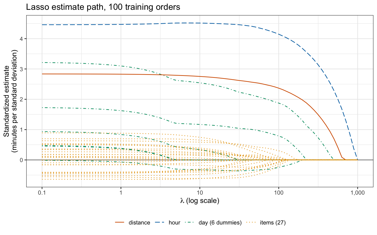
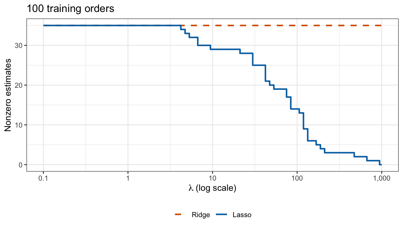
Read from the right. At \(\lambda = 1{,}000\), above \(\lambda_{\max} = 967.4\), every estimate is zero. As \(\lambda\) decreases the first features to enter are hour, distance, and daySat. hour enters at \(\lambda_{\max}\) itself. The grid does not contain the points of entry; the largest grid values of \(\lambda\) at which the three are nonzero are 891, 631, and 447. Each estimate leaves zero continuously rather than jumping to its least squares value. At \(\lambda = 100\), 14 of the 35 estimates are nonzero; at \(\lambda = 10\), 29. On this path no estimate returns to zero once it has entered. An estimate can return to zero when features are correlated; the largest absolute correlation between two of the 35 training features is 0.47. At \(\lambda = 0.1\) all 35 are nonzero, within 0.01 minutes per standard deviation of least squares.

22.4 Tuning parameter selection

22.4.1 Cross-validation

cv.glmnet() computes \(\text{CV}_{(k)}(\lambda)\) on the grid of the path, with \(k = 10\) and the ridge lecture’s folds fold_id; inside each fold glmnet() standardizes from the other 9 folds only. Ridge regression is cross-validated on the same folds and grid as in the ridge lecture.

# Lasso cross-validated on the training folds.
cv_lasso <- cv.glmnet(X_train,
                      y_train,
                      alpha = 1,
                      lambda = to_glmnet(lasso_grid),
                      foldid = fold_id,
                      thresh = 1e-12)
lambda_cv <- to_chapter(cv_lasso$lambda.min)

# Ridge regression cross-validated on the same folds.
cv_ridge <- cv.glmnet(X_train,
                      y_train,
                      alpha = 0,
                      lambda = to_glmnet_ridge(lambda_grid),
                      foldid = fold_id,
                      thresh = 1e-12)
lambda_cv_ridge <- cv_ridge$lambda.min * n_train / s_y

NoteCode

# The ridge lecture's ridge estimate for many lambdas at once, from the
# singular value decomposition of the standardized features. A feature absent
# from a sample gets estimate 0, which at lambda = 0 is least squares on
# the rest; this is the ridge lecture's least squares in every fold and sample.
ridge_path <- function(X, y, lambdas) {
  # Standardize the features, leaving a constant feature unscaled.
  center <- colMeans(X)
  scale <- apply(X, 2, sd_n)
  scale[scale == 0] <- 1
  X_c <- sweep(X, 2, center)
  Z <- sweep(X_c, 2, scale, "/")

  # Shrink each singular direction, one column per lambda.
  sv <- svd(Z)
  shrink <- outer(sv$d, lambdas, \(d, l) ifelse(d > 1e-8, d / (d^2 + l), 0))
  y_centered <- y - mean(y)
  u_y <- drop(crossprod(sv$u, y_centered))
  b <- (sv$v %*% (shrink * u_y)) / scale

  # Intercept, then slopes, on the original scale.
  rbind(`(Intercept)` = mean(y) - colSums(b * center), b)
}

# Least squares MSE on the orders left out of fold l.
ls_fold <- function(l) {
  out <- fold_id == l
  b <- ridge_path(X_train[!out, ], y_train[!out], 0)
  y_hat <- cbind(1, X_train[out, ]) %*% b
  mse(y_train[out], y_hat)
}

# Least squares cross-validation estimate over the same folds.
fold_size <- tabulate(fold_id)
ls_fold_mse <- map_dbl(seq_len(n_folds), ls_fold)
cv_ls <- weighted.mean(ls_fold_mse, fold_size)

# One standard error over the folds, computed as cv.glmnet() computes it.
ls_var <- weighted.mean((ls_fold_mse - cv_ls)^2, fold_size)
ls_se <- sqrt(ls_var / (n_folds - 1))

# Smallest lasso and ridge cross-validation estimates.
cv_lambda <- to_chapter(cv_lasso$lambda)
cv_min <- min(cv_lasso$cvm)
i_min <- which.min(cv_lasso$cvm)
i_min_ridge <- which.min(cv_ridge$cvm)
nonzero_cv <- cv_lasso$nzero[[cv_lasso$index["min", 1]]]

# Grid values whose estimate is within 5% of the smallest.
near_min <- cv_lasso$cvm < 1.05 * cv_min

# Sums of squared errors on the orders left out of fold l, with this
# chapter's lambda applied exactly to the orders the fold is fit to.
fold_sse <- function(l) {
  out <- fold_id == l
  n_in <- sum(!out)
  fit <- glmnet(X_train[!out, ],
                y_train[!out],
                alpha = 1,
                lambda = to_glmnet(lasso_grid, n_in),
                thresh = 1e-12)
  y_hat <- predict(fit, X_train[out, ])
  colSums((y_train[out] - y_hat)^2)
}

# Cross-validation with this chapter's lambda applied exactly in every fold.
fold_sse_all <- sapply(seq_len(n_folds), fold_sse)
cv_exact <- rowSums(fold_sse_all) / n_train

# Cross-validation estimates against lambda, lasso and ridge regression.
method_levels <- c("Lasso", "Ridge regression")
lasso_curve <- tibble(method = method_levels[1],
                      lambda = cv_lambda,
                      cv = cv_lasso$cvm)
ridge_curve <- tibble(method = method_levels[2],
                      lambda = cv_ridge$lambda * n_train / s_y,
                      cv = cv_ridge$cvm)
cv_curves <- bind_rows(lasso_curve, ridge_curve) |>
  mutate(method = factor(method, levels = method_levels))

# The chosen lambda of each, and its estimate, labeled (as plotmath) in the
# empty lower left of each panel.
panel_left <- c(min(lasso_curve$lambda), min(ridge_curve$lambda))
cv_min_ridge <- min(cv_ridge$cvm)
cv_chosen <- tibble(method = factor(method_levels, levels = method_levels),
                    lambda = c(lambda_cv, lambda_cv_ridge),
                    cv = c(cv_min, cv_min_ridge))
chosen_lambda_text <- fmt(cv_chosen$lambda, 1)
chosen_cv_text <- fmt(cv_chosen$cv)
chosen_text <- paste0("'Chosen'~lambda == '", chosen_lambda_text,
                      "'*', estimate ", chosen_cv_text, "'")
chosen_label <- cv_chosen |>
  mutate(label = chosen_text,
         lambda = panel_left,
         cv = cv_min)

# Least squares, lambda = 0, labeled above its line at the left of each panel.
ls_cv_text <- fmt(cv_ls)
ls_label <- tibble(method = factor(method_levels, levels = method_levels),
                   lambda = panel_left,
                   cv = cv_ls,
                   label = paste0("'Least squares'~(lambda == 0)*': ",
                                  ls_cv_text, "'"))

# The two curves, the least squares value, and the chosen lambdas.
cv_plot <- ggplot(cv_curves, aes(x = lambda, y = cv)) +
  geom_hline(yintercept = cv_ls, linetype = "dashed") +
  geom_line(linewidth = 0.8) +
  geom_vline(data = cv_chosen,
             aes(xintercept = lambda),
             linetype = "dotted") +
  geom_point(data = cv_chosen, size = 2.5) +
  geom_text(data = chosen_label,
            aes(label = label),
            parse = TRUE,
            hjust = 0,
            vjust = 0,
            size = 3.5) +
  geom_text(data = ls_label,
            aes(label = label),
            parse = TRUE,
            hjust = 0,
            vjust = -0.6,
            size = 3.5) +
  facet_wrap(~ method, scales = "free_x") +
  log_lambda +
  labs(x = expression(lambda ~ "(log scale)"),
       y = paste0(n_folds, "-fold CV estimate of test MSE"),
       title = paste(n_train, "training orders"))

The figure plots \(\text{CV}_{(10)}(\lambda)\) for the lasso and for ridge regression, each against its own \(\lambda\), with the least squares estimate (\(\lambda = 0\)) as a dashed line and each chosen \(\lambda\) marked.

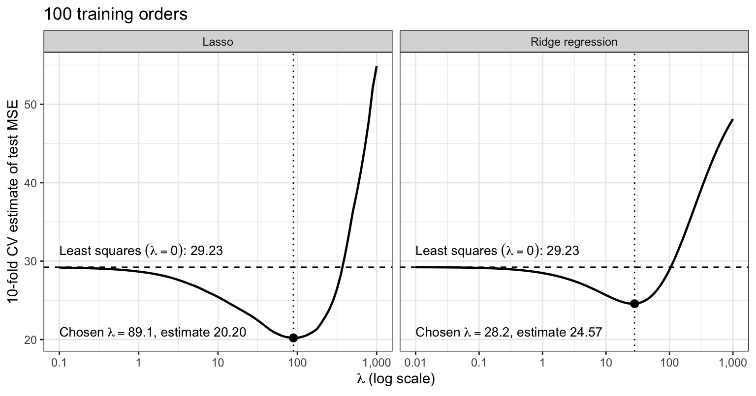
The estimate is smallest, 20.20, at \(\lambda = 89.1\) (\(\lambda_{\text{glmnet}} = 0.446\)), where the lasso estimates of 14 coefficients are nonzero, against 29.23 for least squares and 24.57 for ridge regression at \(\lambda = 28.2\).¹ The minimum is shallow: from \(\lambda = 50\) to 158, with 20 down to 6 nonzero lasso estimates, the cross-validation estimate is within 5% of its smallest value.

Plus or minus one standard error over the folds, the estimate is 16.65 to 23.76 for the lasso at its minimum, 19.62 to 29.52 for ridge regression at its minimum, and 23.51 to 34.95 for least squares, so the lasso and least squares intervals overlap only from 23.51 to 23.76.

22.4.2 Test evaluation

cv.glmnet() has also fit the path to all 100 training orders, so predicting with s = "lambda.min" uses the refit. The three chosen models are evaluated once on the 9,912 test orders.

# Predictions of the three chosen models at the test orders.
lasso_test_pred <- drop(predict(cv_lasso, X_test, s = "lambda.min"))
ridge_test_pred <- drop(predict(cv_ridge, X_test, s = "lambda.min"))
ls_test_pred <- predict(ls_fit, test)

# Test MSE of each.
test_mse <- c(ls = mse(y_test, ls_test_pred),
              ridge = mse(y_test, ridge_test_pred),
              lasso = mse(y_test, lasso_test_pred))

NoteCode

# Training MSE of the three chosen models.
ridge_train_pred <- predict(cv_ridge, X_train, s = "lambda.min")
lasso_train_pred <- predict(cv_lasso, X_train, s = "lambda.min")
ls_train_pred <- fitted(ls_fit)
train_mse <- c(mse(y_train, ls_train_pred),
               mse(y_train, ridge_train_pred),
               mse(y_train, lasso_train_pred))

# Table of lambda, number of nonzero estimates, and the three error
# estimates.
cv_estimates <- c(cv_ls, cv_min_ridge, cv_min)
lambda_text <- c("0", fmt(lambda_cv_ridge, 1), fmt(lambda_cv, 1))
test_columns <- c("Method",
                  "$\\lambda$",
                  "Nonzero estimates",
                  "Training MSE",
                  paste0(n_folds, "-fold CV estimate"),
                  "Test MSE")
test_table <- tibble(Method = c("Least squares", "Ridge", "Lasso"),
                     lambda = lambda_text,
                     kept = c(p, p, nonzero_cv),
                     train = fmt(train_mse),
                     cv = fmt(cv_estimates),
                     test = fmt(test_mse)) |>
  knitr::kable(col.names = test_columns, align = "lrrrrr")

# Paired comparison over the test orders: ridge squared error minus lasso's.
sq_diff <- (y_test - ridge_test_pred)^2 - (y_test - lasso_test_pred)^2

# Cross-validation estimate over test MSE, for least squares, ridge, and
# lasso.
cv_over_test <- cv_estimates / test_mse
stopifnot(all(cv_over_test > 1))

Method	\(\lambda\)	Nonzero estimates	Training MSE	10-fold CV estimate	Test MSE
Least squares	0	35	10.13	29.23	22.02
Ridge	28.2	35	12.23	24.57	20.38
Lasso	89.1	14	13.78	20.20	16.96

The lasso’s test MSE is 16.96, against 20.38 for ridge regression and 22.02 for least squares, 16.8% and 23.0% lower. The paired difference in squared error, ridge minus lasso, has mean 3.42 and standard error 0.16 over the test orders. As in the ridge lecture, that standard error treats the fitted models as fixed and says nothing about another training sample; the repeated samples below do.

All three cross-validation estimates are above the test MSEs, by factors of 1.19 to 1.33. As in the ridge lecture, each fit in cross-validation uses 90 orders, and with so few orders per feature the error falls quickly as orders are added; an estimate from 100 orders is also noisy. The lasso and ridge estimates are, in addition, each the smallest over a grid of \(\lambda\) values, selected for being low, so as estimates of the chosen model’s error they are optimistic. The least squares estimate involves no such choice.

22.4.3 Lasso estimates

NoteCode

# Estimates of the three chosen models on the original scale.
b_lasso <- coef(cv_lasso, s = "lambda.min")[, 1]
b_ridge <- coef(cv_ridge, s = "lambda.min")[, 1]
b_ls <- coef(ls_fit)

# One row per feature and fit.
feature_order <- colnames(X_train)
feature_levels <- rev(feature_order)
fit_labels <- c("Least squares", "Ridge", "Lasso")
feature_rep <- rep(feature_order, 3)
fit_rep <- rep(fit_labels, each = p)
fit_estimates <- tibble(
  feature = factor(feature_rep, levels = feature_levels),
  estimate = c(b_ls[feature_order],
               b_ridge[feature_order],
               b_lasso[feature_order]),
  fit = factor(fit_rep, levels = fit_labels)
)

# The estimates of the three fits, feature by feature.
estimate_plot <- ggplot(fit_estimates,
                        aes(x = estimate,
                            y = feature,
                            color = fit,
                            shape = fit)) +
  geom_vline(xintercept = 0, linetype = "dotted") +
  geom_point(size = 2, position = position_dodge(width = 0.7)) +
  scale_color_manual(values = okabe_ito[c(1, 4, 5)]) +
  scale_shape_manual(values = c(1, 17, 16)) +
  labs(x = "Estimate (minutes per unit of the feature)",
       y = NULL,
       color = NULL,
       shape = NULL,
       title = paste(n_train, "training orders")) +
  theme(legend.position = "bottom")

# The features the lasso keeps, by kind.
kept <- names(b_lasso)[-1][b_lasso[-1] != 0]
kept_items <- intersect(kept, item_names)
day_names <- feature_order[str_starts(feature_order, "day")]
kept_days <- intersect(kept, day_names)
dropped_days <- str_remove(setdiff(day_names, kept), "day")

# Kept items with positive and with negative estimates, largest first.
b_items <- b_lasso[kept_items]
items_pos <- sort(b_items[b_items > 0], decreasing = TRUE)
items_neg <- sort(b_items[b_items < 0])

# Predicted time of a Monday order with no items at the training orders'
# mean hour and mean distance.
typical_x <- c(1, mean(train$hour), mean(train$distance))
typical <- sum(b_lasso[c("(Intercept)", "hour", "distance")] * typical_x)

# Nonzero lasso estimates smaller in absolute value than least squares'.
n_shrunk <- sum(abs(b_lasso[kept]) < abs(b_ls[kept]))

The figure compares the estimates of the three fits, on the original scale.

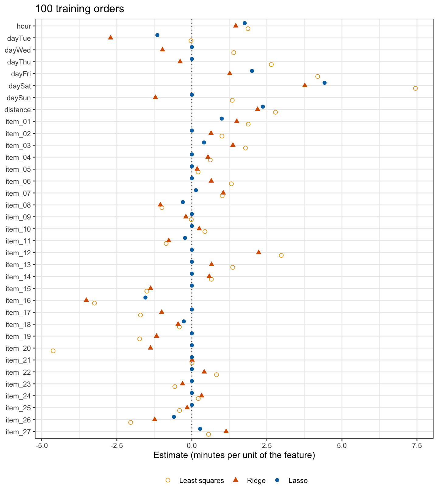
Read in order,

• Intercept. On the original scale, \(\hat\beta_0 = -10.5\) minutes is the predicted time of a Monday order placed at hour 0, at distance 0, with no items, far outside the data. (The standardized-scale intercept is \(\bar y = 26.7\) minutes.) A Monday order with no items at the training orders’ mean hour, 16.2, and mean distance, 3.05 miles, has predicted time 25.3 minutes.
• Hour and distance. Each hour later adds 1.76 minutes (ridge 1.46, least squares 1.87), and each mile 2.37 minutes (ridge 2.19, least squares 2.79), holding the other features fixed. Relative to least squares, ridge regression shrinks the two by 22% and 21%, the lasso by 6% and 15%.
• Day. The lasso keeps the dummies for Tue, Fri, and Sat, with estimates −1.1, 2.0, and 4.4 minutes, and drops those for Wed, Thu, and Sun. As in the Subset Selection lecture, a dropped dummy merges its day into the reference: the model predicts Wed, Thu, and Sun orders like otherwise identical Monday orders.
• Items. The lasso keeps 9 of the 27 items. Each unit of item_01, item_03, item_27, and item_07 raises the predicted time, by 1.00, 0.41, 0.28, and 0.13 minutes, and each unit of item_16, item_26, item_08, item_18, and item_11 lowers it, by 1.55, 0.60, 0.30, 0.27, and 0.23 minutes. The other 18 items do not affect the prediction. These signs are read with care: item_16, with the most negative item estimate, is in only 3 of the training orders, and the repeated samples below show how much the kept items depend on the training sample.

Of the 14 nonzero lasso estimates, 13 are smaller in absolute value than their least squares counterparts. Nonzero lasso estimates are shrunken toward zero, by \(\lambda/(2n)\) in the orthogonal case, so the lasso estimator, the rule that turns a training sample into an estimate, is biased toward zero for a nonzero coefficient, as the repeated samples below show. And because the features were selected using the same data, the standard errors, \(t\)-statistics, and \(p\)-values that lm() would report, for the lasso fit or for least squares refit to the selected features, do not apply, as in the subset selection lecture. glmnet() reports none.

22.5 Repeated training samples

22.5.1 Test MSE

# Number of training samples of each size, and number of test orders at
# which every prediction is made.
n_samples <- 500
n_predict <- 4000

As in the ridge lecture, 4,000 of the 9,912 test orders are the test orders at which every prediction is made, and the remaining 5,912 test orders are the orders from which the repeated training samples are drawn: \(M = 500\) samples of \(n\) of the remaining test orders. These random draws repeat, in the same order, those of the ridge lecture, so the samples and the folds drawn within each are identical in the two lectures. In each sample \(\lambda\) is chosen by 10-fold cross-validation, for the lasso and for ridge regression on the same folds, each is refit, and its MSE at the 4,000 test orders is compared with that of least squares fit to the same sample, for \(n = 100\) and \(n = 300\).

NoteCode

# Divide the test orders: those at which every prediction is made, and the
# remaining test orders, from which the training samples are drawn.
predict_rows <- sample(n_test, n_predict)
test_predict <- test[predict_rows, ]
test_rest <- test[-predict_rows, ]
X_predict <- model_matrix(test_predict)
y_predict <- test_predict$time_to_delivery
X_rest <- model_matrix(test_rest)
y_rest <- test_rest$time_to_delivery

# Training samples of n_train and of n_large of the remaining test orders.
n_rest <- nrow(test_rest)
sample_ids <- map(seq_len(n_samples), \(s) sample(n_rest, n_train))
sample_ids_large <- map(seq_len(n_samples), \(s) sample(n_rest, n_large))

# Fit least squares, ridge regression, and the lasso to one training sample,
# with lambda chosen by cross-validation on the same folds for both
# penalties, and compute each fit's MSE at the test orders.
fit_sample <- function(id) {
  # The training sample and its folds.
  X <- X_rest[id, ]
  y <- y_rest[id]
  n <- length(y)
  fold_labels <- rep(seq_len(n_folds), length.out = n)
  folds <- sample(fold_labels)

  # Ridge regression and the lasso, cross-validated.
  cv_r <- cv.glmnet(X,
                    y,
                    alpha = 0,
                    lambda = lambda_grid * sd_n(y) / n,
                    foldid = folds,
                    thresh = 1e-10)
  cv_l <- cv.glmnet(X,
                    y,
                    alpha = 1,
                    lambda = to_glmnet(lasso_grid, n),
                    foldid = folds,
                    thresh = 1e-10)

  # Estimates of the three fits on the original scale.
  ls_estimates <- ridge_path(X, y, 0)[, 1]
  estimate_names <- c("(Intercept)", colnames(X))
  b_ls_s <- setNames(ls_estimates, estimate_names)
  b_lasso_s <- coef(cv_l, s = "lambda.min")[, 1]
  b_ridge_s <- coef(cv_r, s = "lambda.min")[, 1]

  # Predictions at the test orders.
  ls_pred <- cbind(1, X_predict) %*% b_ls_s
  ridge_pred <- predict(cv_r, X_predict, s = "lambda.min")
  lasso_pred <- predict(cv_l, X_predict, s = "lambda.min")

  # MSEs, the features the lasso keeps, and the hour and distance estimates.
  two_estimates <- tibble(feature = c("hour", "distance"),
                          `Least squares` = b_ls_s[feature],
                          Ridge = b_ridge_s[feature],
                          Lasso = b_lasso_s[feature])
  tibble(n = n,
         ls = mse(y_predict, ls_pred),
         ridge = mse(y_predict, ridge_pred),
         lasso = mse(y_predict, lasso_pred),
         kept = list(b_lasso_s[-1] != 0),
         estimates = list(two_estimates))
}

# Fit every training sample of one size, one row per sample.
fit_samples <- function(ids) {
  map(ids, fit_sample) |>
    list_rbind()
}

# Both sizes, in this order, so the folds are the ridge lecture's.
reps_small <- fit_samples(sample_ids)
reps_large <- fit_samples(sample_ids_large)
reps <- bind_rows(reps_small, reps_large)

# Share of samples in which one method beats another, and average MSEs.
rep_summary <- reps |>
  group_by(n) |>
  summarize(lasso_beats_ls = mean(lasso < ls),
            lasso_beats_ridge = mean(lasso < ridge),
            ridge_beats_ls = mean(ridge < ls),
            mse_ls = mean(ls),
            mse_ridge = mean(ridge),
            mse_lasso = mean(lasso))

# One summary for one sample size.
rs <- function(size, col) {
  rep_summary[[col]][rep_summary$n == size]
}

# Per-sample gain over least squares with n = 100, and where this training
# sample's test gain falls among them.
reps_100 <- filter(reps, n == n_train)
sample_gain <- 1 - reps_100$lasso / reps_100$ls
test_gain <- 1 - test_mse[["lasso"]] / test_mse[["ls"]]
gain_range <- quantile(sample_gain, c(0.05, 0.95))

# Percent change in MSE relative to least squares, per sample.
size_labels <- paste("n =", c(n_train, n_large))
rep_changes <- reps |>
  mutate(size = paste("n =", n)) |>
  transmute(n = factor(size, levels = size_labels),
            Ridge = 100 * (ridge / ls - 1),
            Lasso = 100 * (lasso / ls - 1)) |>
  pivot_longer(-n, names_to = "method", values_to = "change") |>
  mutate(method = factor(method, levels = ridge_lasso))

# Their distribution for each method and sample size.
rep_y <- paste0("Change in MSE at the ", big(n_predict), " test orders\n",
                "relative to least squares (%)")
rep_plot <- ggplot(rep_changes, aes(x = method, y = change)) +
  geom_hline(yintercept = 0, linetype = "dashed", color = "grey50") +
  geom_violin(fill = "grey90",
              scale = "width",
              quantiles = c(0.25, 0.5, 0.75),
              quantile.linetype = "solid") +
  facet_wrap(~ n) +
  labs(x = NULL,
       y = rep_y,
       title = paste(n_samples, "training samples of each size"),
       caption = paste("Lines = quartiles and median;",
                       "below 0 = better than least squares."))

The figure plots, for each sample, the percent change in MSE at the 4,000 test orders relative to least squares.

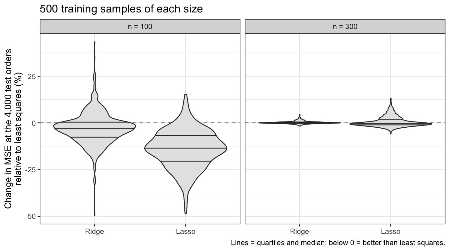
With \(n = 100\) the average MSE is 19.19 for the lasso, 21.74 for ridge regression, and 22.58 for least squares. The lasso has a lower MSE than least squares in 94% of the samples and than ridge regression in 94%; ridge regression beats least squares in 72%, the ridge lecture’s figure. On these data, with 100 training orders, the lasso’s advantage is not an accident of one training sample, although its average MSE, 15.0% below that of least squares, is a smaller gain than the 23.0% on the test orders.

This training sample is a favorable draw for the lasso. The median gain over the samples is 13.5%, 90% of the gains lie between −1.9% and 31.5%, and 18.4% of the samples gain at least as much as this one, which puts it at about the 82nd percentile.

With \(n = 300\) the averages are 16.04, 15.97, and 15.94. The lasso beats least squares in 56% of the samples, but its average MSE is 0.6% above that of least squares: it loses less often than it wins, but by more. With 300 orders least squares has little variance left to remove, and neither penalty improves on it on average.

22.5.2 Selected sets

NoteCode

# Which features the lasso keeps, one row per training sample.
reps_300 <- filter(reps, n == n_large)
kept_100 <- do.call(rbind, reps_100$kept)
kept_300 <- do.call(rbind, reps_300$kept)

# Share of samples in which the lasso keeps each feature.
share_100 <- colMeans(kept_100)
share_300 <- colMeans(kept_300)
share_features <- rep(feature_order, 2)
size_rep <- rep(size_labels, each = p)
keep_shares <- tibble(
  feature = factor(share_features, levels = feature_levels),
  share = c(share_100, share_300),
  n = factor(size_rep, levels = size_labels)
)

# Feature labels, starred if the lasso fit to the training orders keeps them.
mark_kept <- function(f) {
  if_else(f %in% kept, paste0(f, " *"), f)
}

# The shares, one row per feature.
freq_plot <- ggplot(keep_shares,
                    aes(x = share,
                        y = feature,
                        color = n,
                        shape = n)) +
  geom_point(size = 2) +
  scale_x_continuous(labels = scales::percent, limits = c(0, 1)) +
  scale_y_discrete(labels = mark_kept) +
  scale_color_manual(values = okabe_ito[c(5, 4)]) +
  scale_shape_manual(values = c(16, 17)) +
  labs(x = "Share of samples in which the lasso keeps the feature",
       y = NULL,
       color = NULL,
       shape = NULL,
       title = paste(n_samples, "training samples of each size"),
       caption = "* = kept by the lasso fit to the training orders.") +
  theme(legend.position = "bottom")

# Number of features kept per sample, and the items kept most often.
size_100 <- rowSums(kept_100)
item_share <- colMeans(kept_100[, item_names])
top_share <- names(sort(item_share, decreasing = TRUE))[1:2]
top_item <- names(which.max(item_share))
neg_item <- names(items_neg)[1]

# A reference outside the workflow: the least squares fit to the test orders
# at which every prediction is made. It uses test orders to fit a model, so
# it tests nothing.
ref_fit <- lm(time_to_delivery ~ ., data = test_predict)
ref_coefs <- summary(ref_fit)$coefficients[item_names, ]
ref_slow <- ref_coefs[, "Estimate"] > 0 & ref_coefs[, "Pr(>|t|)"] < 0.05
ref_top <- names(sort(ref_coefs[, "Estimate"], decreasing = TRUE))[1:2]

The figure plots how often the lasso kept each feature over the samples.

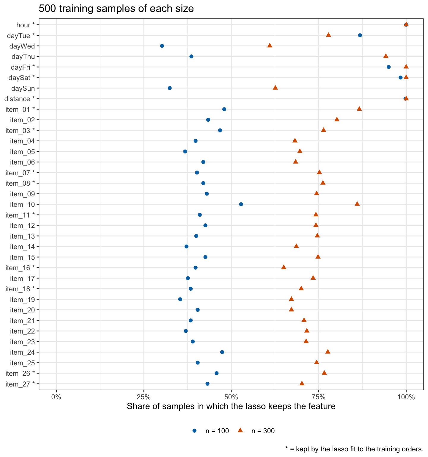
With \(n = 100\), hour and distance are kept in 100.0% and 99.8% of the samples and each item in between 35% and 53%. The lasso keeps a median of 16 features, from 4 to 35, and the 500 samples give 494 different selected sets. With \(n = 300\) it keeps more, a median of 29, and each item in more samples.

The selected items are not the only items that slow deliveries. The least squares fit to the 4,000 test orders uses test orders to fit a model, so it is a reference outside the workflow and not a test of anything. It gives 25 of the 27 items a positive estimate with \(p\)-value below 0.05, a median of 0.6 minutes per item, the largest for item_01 and item_10, the two items the lasso keeps most often; even item_10 is kept in only 53% of the samples. The lasso fit to the training orders drops item_10 and gives item_16 its most negative item estimate, −1.55 minutes, where the least squares fit to the 4,000 test orders gives 0.27 (\(p\)-value 0.28). Of the 5 items with negative estimates in the lasso fit to the training orders, 4 have a positive estimate with \(p\)-value below 0.05 in the least squares fit to the 4,000 test orders. Almost every item slows deliveries a little; with 100 orders those small effects are estimated with large error, and which of them clear the threshold depends on the noise in the sample. A dropped item is not shown to have no effect.

22.5.3 Estimator bias

NoteCode

# Hour and distance estimates of the three fits to each training sample of
# n_train orders.
two_levels <- c("hour", "distance")
estimate_reps <- reps_100$estimates |>
  list_rbind() |>
  pivot_longer(-feature, names_to = "fit", values_to = "estimate") |>
  mutate(fit = factor(fit, levels = fit_labels),
         feature = factor(feature, levels = two_levels))

# The least squares fit to the test orders, a reference outside the workflow.
ref_ls <- coef(ref_fit)[two_levels]

# Average estimate of each fit, for hour and distance.
estimate_means <- estimate_reps |>
  group_by(feature, fit) |>
  summarize(mean = mean(estimate), .groups = "drop")
cmean <- function(f, m) {
  estimate_means$mean[estimate_means$feature == f & estimate_means$fit == m]
}

# Average shrinkage relative to the least squares average, hour then
# distance.
avg_shrink <- function(m) {
  ratio <- map_dbl(two_levels, \(f) cmean(f, m) / cmean(f, "Least squares"))
  1 - ratio
}

# The prose says ridge regression shrinks both more than the lasso, on
# average and in the fit to the training orders.
shrink_ridge <- avg_shrink("Ridge")
shrink_lasso <- avg_shrink("Lasso")
stopifnot(all(shrink_ridge > shrink_lasso),
          all(shrink_lasso > 0),
          all(b_ridge[two_levels] < b_lasso[two_levels]))

# The estimates over the samples, with the reference values as lines.
ref_lines <- tibble(feature = factor(two_levels, levels = two_levels),
                    estimate = ref_ls)
feature_labels <- as_labeller(c(hour = "hour (minutes per hour)",
                                distance = "distance (minutes per mile)"))
bias_title <- paste(n_samples, "training samples of", n_train,
                    "remaining test orders")
bias_caption <- paste0("Lines = quartiles and median; diamond = mean;\n",
                       "dashed line = least squares fit to the ",
                       big(n_predict), " test orders.")
bias_plot <- ggplot(estimate_reps, aes(x = fit, y = estimate)) +
  geom_violin(fill = "grey90",
              scale = "width",
              quantiles = c(0.25, 0.5, 0.75),
              quantile.linetype = "solid") +
  stat_summary(fun = mean, geom = "point", shape = 18, size = 3) +
  geom_hline(data = ref_lines,
             aes(yintercept = estimate),
             linetype = "dashed",
             color = okabe_ito[4]) +
  facet_wrap(~ feature, scales = "free_y", labeller = feature_labels) +
  labs(x = NULL,
       y = "Estimate",
       title = bias_title,
       caption = bias_caption)

Bias is a property of an estimator, not of the estimates from one sample: it is the difference between the average of the estimates over repeated training samples and the coefficient they estimate. The figure plots the estimates of the hour and distance coefficients, on the original scale, from the three fits to each of the 500 training samples of 100 of the remaining test orders. The dashed lines are the estimates of the least squares fit to the 4,000 test orders, the reference outside the workflow described in the previous subsection.

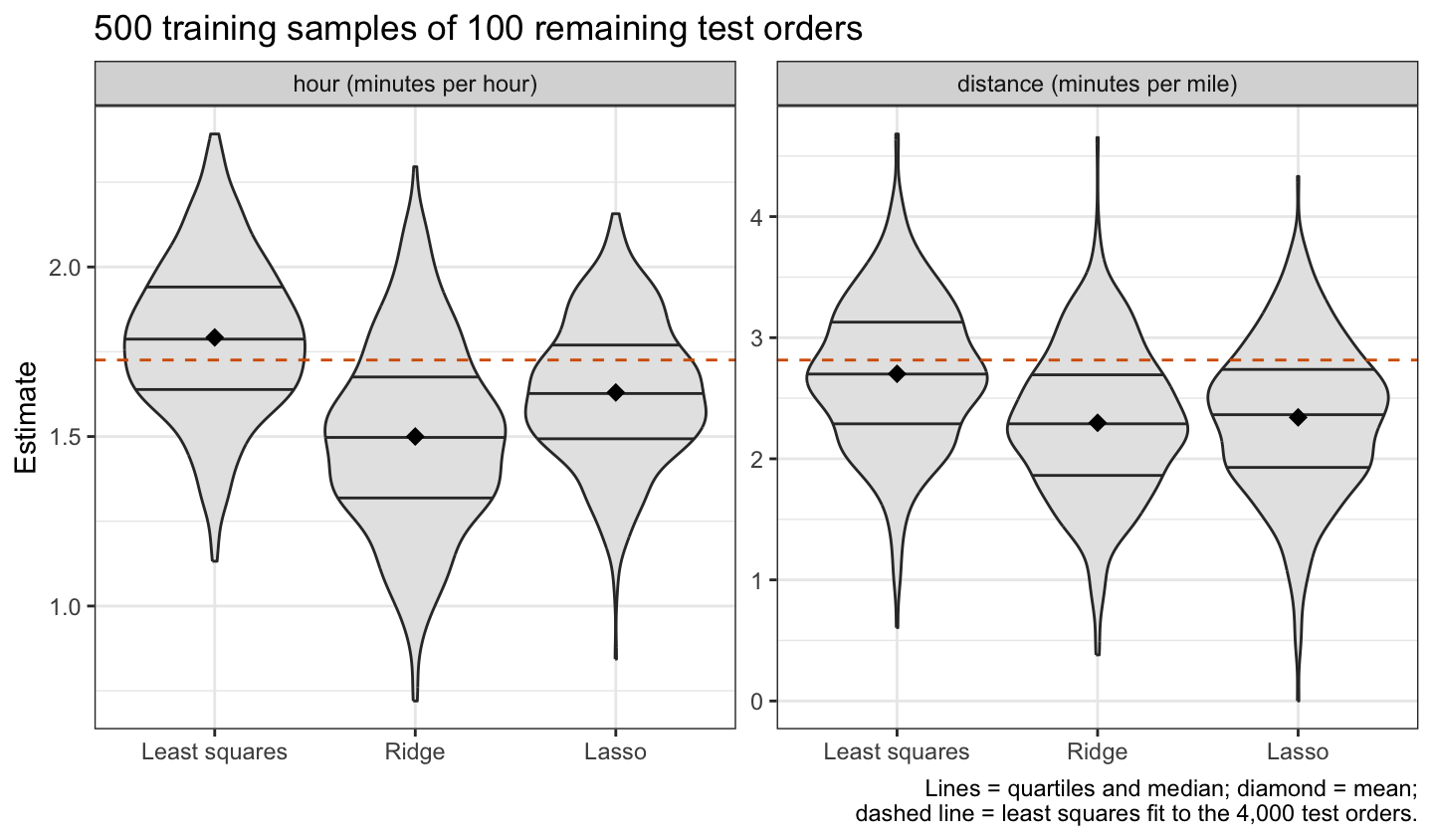
Over the samples, least squares averages 1.79 minutes per hour and 2.70 per mile, close to the 1.73 and 2.82 of the least squares fit to the 4,000 test orders. The lasso averages 1.63 and 2.34 (zeros included), 9% and 13% below the least squares averages: the lasso estimators of the hour and distance coefficients are biased toward zero. Ridge regression averages 1.50 and 2.30, 16% and 15% below.

The lasso plausibly predicts better than ridge regression on these data for two reasons. It sets to zero the item estimates too noisy to help the predictions. And ridge regression has one \(\lambda\) for all 35 coefficients: a \(\lambda\) large enough to shrink the noisy item estimates also shrinks the large hour and distance estimates more than the lasso does, in the fit to the training orders and on average over the samples. Neither reason has been isolated from the other here.

Which penalty predicts better depends on how many features carry the signal. The reasoning above suggests the lasso predicts better when a few features matter and the rest are noise, and ridge regression when many features have small effects of similar size, because the lasso then sets real signal to zero. One dataset cannot show that.

NoteBeyond this course

• Bayesian interpretation. If \(y_i \mid \beta \stackrel{ind}{\sim} N\left(\beta_0 + \tilde x_i\beta, \sigma^2\right)\), with \(\tilde x_i\) row \(i\) of \(\tilde{\mathbf{X}}\), and the slopes have independent Laplace priors with density proportional to \(\exp\left(-\left|\beta_j\right|/b\right)\) (and a flat prior on \(\beta_0\)), the posterior mode of \(\beta\) is the lasso estimate with \(\lambda = 2\sigma^2/b\). Ridge regression’s normal prior gives a posterior whose mode and mean coincide.
• Elastic net. glmnet()’s alpha between 0 and 1 mixes the two penalties, keeping some of the lasso’s zeros while sharing weight among correlated features as ridge regression does.
• One-standard-error rule. cv.glmnet()’s lambda.1se, the largest \(\lambda\) whose cross-validation estimate is within one standard error of the smallest, here \(\lambda = 223.9\) with 3 nonzero lasso estimates, chooses a smaller model where the curve is flat.
• Group lasso. The lasso treats the 6 day dummies as separate features, so it can keep some and drop others, as it did here. The group lasso penalizes the length of each group of coefficients, so it keeps or drops all the dummies of one categorical explanatory variable together.
• Inference after selection. Methods exist for valid confidence intervals and tests after lasso selection, under assumptions this course does not cover.

22.6 Conclusion

The lasso estimates the coefficients of standardized features by minimizing \(RSS + \lambda\sum_{j=1}^p\left|\beta_j\right|\), with the intercept unpenalized. Equivalently, it minimizes the RSS within the budget \(\sum_j\left|\beta_j\right| \le s\), a region with corners and edges on which some \(\beta_j\) are zero. A set of least squares estimates with positive volume leads to each of them, so some lasso estimates are exactly zero. Ridge regression’s disk \(\sum_j\beta_j^2 \le s\) has no corners, the least squares estimates that give a zero ridge estimate form a set of zero volume, and its estimates are shrunken but, except by coincidence, not zero. Best subset selection is the same problem with a budget on the number of nonzero coefficients, the \(\ell_0\) penalty; the lasso is its convex relaxation.

The lasso has no closed form in general. For orthogonal standardized features it soft-thresholds the least squares estimate, moving each estimate toward zero by \(\lambda/(2n)\) and setting to zero those within that distance, where ridge regression multiplies each by \(n/(n + \lambda)\); in general it is computed by coordinate descent, one soft-thresholding step per coefficient. Its estimate path starts from the null model at \(\lambda_{\max}\) and adds features as \(\lambda\) decreases, and the number of nonzero estimates plays the role of the model size \(d\) of subset selection. glmnet()’s \(\lambda\) converts to this one by \(\lambda = 2n\lambda_{\text{glmnet}}\).

\(\lambda\) is chosen by \(k\)-fold cross-validation on the training data, with the standardization repeated inside every fold, followed by a refit, and the chosen model is evaluated once on test data. The smallest cross-validation estimate is optimistic as an estimate of the chosen model’s error, because \(\lambda\) was chosen to make it small. Whether the lasso predicts better than ridge regression or least squares depends on the data and the training sample size, and is best judged over repeated samples rather than one. The lasso is expected to predict better when a few features carry the signal and ridge regression when many features have small effects of similar size, but one dataset cannot show that. The set of features it selects can change from sample to sample, especially when many features have small effects of similar size, so a dropped feature is not shown to have no effect. The nonzero lasso estimates are shrunken toward zero, the lasso estimator of a nonzero coefficient is biased toward zero, and lm()’s standard errors and \(p\)-values do not apply to the lasso estimates.

The next lecture begins dimension reduction with principal components: directions of maximum variance in the features, their loadings and scores, and the proportion of variance each explains.

---

1. Each fold is fit to 90 orders, so by \(\lambda = 2n\lambda_{\text{glmnet}}\) the \(\lambda\) a fold applies is 0.90 times the plotted value, which uses all 100 training orders. Applying this chapter’s \(\lambda\) exactly in every fold gives a smallest estimate of 20.21 at \(\lambda = 79.4\); no conclusion below changes.