13 Linear Discriminant Analysis

Learning objectives

After this lecture you should be able to

derive the posterior probability $p_k(x) = P(Y = k \mid X = x)$ from the prior probabilities $\pi_k$ and the class-conditional densities $f_k(x)$ using Bayes’ theorem, and explain why classifying to the class with the largest posterior probability minimizes the expected error rate,
derive the LDA discriminant function $\delta_k(x)$ for one feature under Gaussian class-conditional densities with a shared variance $\sigma^2$, and show that it is linear in $x$, so that the decision boundary is a single point that moves toward, and when the prior is small enough past, the mean of the class whose prior probability is smaller,
write the discriminant function for $p > 1$ features in matrix form using class mean vectors $\mu_k$ and a shared covariance matrix $\Sigma$, and compute the estimates $\hat\pi_k$, $\hat\mu_k$, and $\hat\sigma^2$ or $\hat\Sigma$ from training data,
fit LDA with MASS::lda(), interpret its prior probabilities, group means, and posterior probabilities, and compare its posterior probabilities and decision boundary with those of logistic regression.

13.1 Generative classifiers

13.1.1 Credit card default data

Question. How does a classifier built from how balance and income are distributed within defaulters and within non-defaulters assign credit card customers to classes, and how do its posterior probabilities and decision boundary compare with those of logistic regressions fit to the same customers and features?

These customers were analyzed in the logistic regression lectures: the Simple Logistic Regression lecture modeled default from balance, the Multiple Logistic Regression lecture from balance and student, and the Flexible Logistic Regression lecture added interactions, including one between balance and income.

Data. ISLR2::Default is a simulated data set of 10,000 credit card customers. The response is default, with Yes the positive class. This lecture uses the two quantitative explanatory variables, balance, the customer’s monthly credit card balance in dollars, and income, the customer’s income in dollars, because linear discriminant analysis (LDA), the method of this lecture, models each class’s features with a Gaussian density. The features are the explanatory variables themselves. income enters the models in dollars as recorded, as in the flexible logistic regression lecture; its coefficients are reported here per $1,000 of income. student (Yes/No) explains the bimodal income distribution in the Multiple-feature LDA section.

The table gives each default class’s number and proportion of customers and the mean, standard deviation, and number of zero values of its balances. The first tab below shows balance within each class, one panel per class, on the density scale; the second shows all customers in one histogram on the count scale, with each bar split into non-defaulters (light blue) and defaulters (dark orange).

Code

Default <- Default |>
  mutate(default01   = as.numeric(default == "Yes"),
         default_jit = default01 + runif(n(), -0.03, 0.03))

dollars <- function(v) format(round(v), big.mark = ",")
# Axis labels such as $60,000, without the scales package.
dollar_labels <- function(v) {
  ifelse(is.na(v), NA,
         paste0("$", format(v, big.mark = ",", scientific = FALSE, trim = TRUE)))
}

class_summary <- Default |>
  group_by(default) |>
  summarize(n = n(), prop = n() / nrow(Default),
            mean_balance = mean(balance), sd_balance = sd(balance),
            n_zero = sum(balance == 0), .groups = "drop")
summary_of <- function(k, col) class_summary[[col]][class_summary$default == k]

class_summary_table <- class_summary |>
  transmute(default, n = format(n, big.mark = ","),
            prop = sprintf("%.4f", prop),
            mean_balance = dollars(mean_balance),
            sd_balance = dollars(sd_balance),
            n_zero = format(n_zero, big.mark = ",")) |>
  knitr::kable(col.names = c("Default", "Customers", "Proportion",
                             "Mean balance (\\$)", "SD of balance (\\$)",
                             "Zero balances"),
               align = "cccccc")

balance_hist_plot <- ggplot(Default, aes(x = balance)) +
  geom_histogram(aes(y = after_stat(density)), binwidth = 100,
                 boundary = 0, fill = "grey80", color = "grey55") +
  facet_wrap(~ default, ncol = 1, labeller = label_both) +
  scale_x_continuous(labels = dollar_labels) +
  labs(x = "Credit card balance ($)", y = "Density",
       title = "ISLR2::Default, balance within each default class")

# All customers on the count scale, each bar split by default status. The
# fills differ in lightness so the split survives without color.
balance_stack_plot <- ggplot(Default, aes(x = balance, fill = default)) +
  geom_histogram(binwidth = 100, boundary = 0, color = "grey30",
                 linewidth = 0.2) +
  scale_fill_manual(values = c(No = "#9DC3E6", Yes = "#D55E00")) +
  scale_x_continuous(labels = dollar_labels) +
  labs(x = "Credit card balance ($)", y = "Customers", fill = "Default",
       title = "ISLR2::Default, all customers by default status")

# Share of defaulters in each $100 balance bin holding at least min_bin_n
# customers.
bin_width <- 100
min_bin_n <- 10
example_bin <- 2000
bin_share <- Default |>
  mutate(bin = floor(balance / bin_width) * bin_width) |>
  group_by(bin) |>
  summarize(n = n(), share = mean(default == "Yes"), .groups = "drop") |>
  filter(n >= min_bin_n)
share_at <- function(b) bin_share$share[bin_share$bin == b]
first_majority_bin <- min(bin_share$bin[bin_share$share > 0.5])

Default	Customers	Proportion	Mean balance ($)	SD of balance ($)	Zero balances
No	9,667	0.9667	804	456	499
Yes	333	0.0333	1,748	341	0

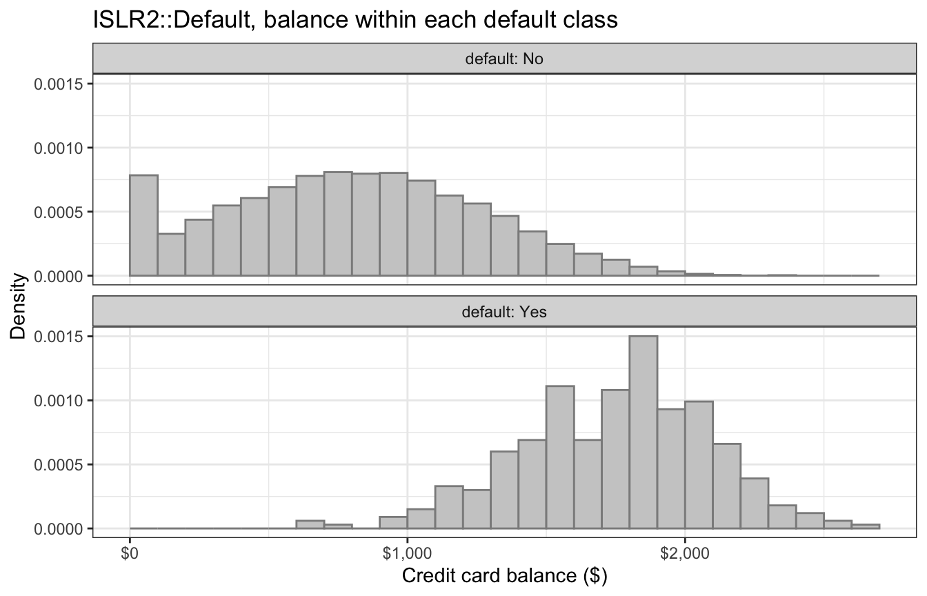
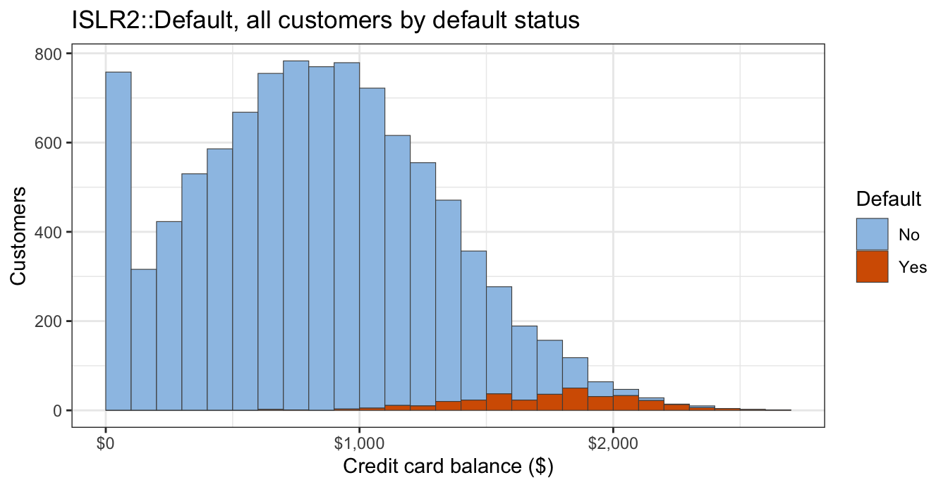
Only 333 customers, a proportion of 0.0333, defaulted. Within each class the balances form a single, roughly bell-shaped pile, and the two piles are centered at different values: defaulters average $1,748 against $804 for non-defaulters. The standard deviations, $456 for non-defaulters and $341 for defaulters, are of the same order but not equal, and the non-defaulter histogram has a spike at zero: 499 customers carry no balance, and no defaulter does.

On the count scale, defaulters are a thin layer at the bottom of the bars at most balances and make up most of a bar only at the largest balances.

13.1.2 Bayes’ theorem

With the response falling in one of $K$ classes, indexed $k = 1, \ldots, K$, logistic regression models the conditional probability $P(Y = k \mid X = x)$ directly. Its likelihood is the conditional distribution of the response given the features, and the distribution of the features themselves never enters it.

A generative classifier takes the other route. It models how the features are distributed within each class, as in the first tab above, and how common each class is, and then reverses the conditioning with Bayes’ theorem to obtain $P(Y = k \mid X = x)$. LDA is the first generative classifier in this course.

Every earlier lecture conditioned on the features and treated them as fixed. A generative classifier models their distribution, so here $X$ is a random vector — the features of a randomly chosen observation — and $x$ is a value it takes. With $Y$ the response, define

\[\pi_k = P(Y = k), \qquad f_k(x) = \text{density of } X \text{ given } Y = k,\]

where

$K$ is the number of classes ($K = 2$ for a binary response),
$\pi_k$ is the prior probability of class $k$, the probability that a randomly chosen observation belongs to class $k$ before its features are seen, with $\sum_{k=1}^K \pi_k = 1$, and
$f_k(x)$ is the class-conditional density of $X$ among observations in class $k$ (a probability mass function if $X$ is discrete).

The classification and logistic regression lectures wrote $C$ for the number of classes; following ISLR2, this and later lectures write $K$.

Bayes’ theorem, with densities in place of the probabilities of the events $\{X = x\}$, gives

\[P(Y = k \mid X = x) = \frac{P(Y = k)\, f_k(x)}{f(x)},\]

where $f(x)$ is the marginal density of $X$. By the law of total probability, $f(x) = \sum_{l=1}^K P(Y = l)\, f_l(x)$, so

\[p_k(x) = P(Y = k \mid X = x) = \frac{\pi_k f_k(x)}{\sum_{l=1}^K \pi_l f_l(x)} \propto \pi_k f_k(x),\]

where

$p_k(x)$ is the posterior probability of class $k$ for an observation with features $x$,
$l$ indexes the classes in the sum, kept distinct from the $k$ being evaluated, and
$\propto$ means “proportional to” as a function of $k$ at a fixed $x$.

Only the numerator distinguishes one class from another: a class is probable at $x$ when it is common ($\pi_k$ large) and when $x$ is a typical feature value for it ($f_k(x)$ large).

For the credit card customers the class proportions estimate the priors, $\hat\pi_{\text{No}} = 0.9667$ and $\hat\pi_{\text{Yes}} = 0.0333$, and the two panels of the first tab picture $f_{\text{No}}$ and $f_{\text{Yes}}$ for balance. The second tab pictures the numerators: each colored segment’s height is proportional to $\pi_k f_k(x)$ over its bin, the whole bar’s to their sum $f(x)$, and the defaulters’ share of the bar estimates $p_{\text{Yes}}(x)$. Among customers with balances from $2,000 to $2,100, for example, a share of 0.702 defaulted.

13.1.3 Bayes classifier

A classifier is an assignment rule $\hat y(x)$ that maps each value of the features to one of the classes $1, \ldots, K$. The Bayes classifier assigns each observation to the class with the largest posterior probability,

\[\hat y(x) = \arg\max_k\, p_k(x),\]

where

$\hat y(x)$ is the class assigned to an observation with features $x$, and
$\arg\max_k p_k(x)$ is the class $k$ at which $p_k(x)$ is largest.

With $K = 2$ classes, $p_1(x) = 1 - p_2(x)$, so the Bayes classifier assigns class $2$ whenever $p_2(x) > 0.5$.

For any classifier, the probability that the assignment at $x$ is wrong is

\[P\left(Y \ne \hat y(x) \mid X = x\right) = 1 - p_{\hat y(x)}(x).\]

This is smallest when $p_{\hat y(x)}(x)$ is largest, which is exactly the Bayes classifier’s choice. The Bayes classifier therefore minimizes the conditional error probability at every $x$, and so it also minimizes the overall error rate $E\left[1 - p_{\hat y(X)}(X)\right]$, which averages those conditional error probabilities over the distribution of $X$. Its overall error rate, the Bayes error rate, is the lowest achievable by any classifier.

An estimate of this rule from the bars of the stacked histogram assigns Yes where defaulters make up more than half a bar, which first happens in the bin starting at $2,000 (among bins with at least 10 customers). With no feature information the largest posterior probability is the largest prior, so every customer would be assigned No, and the 3.33% who defaulted would all be misclassified; that error rate is the one any classifier using features has to beat.

The Bayes classifier needs the true $\pi_k$ and $f_k$, which are never known. A generative classifier estimates both from training data and substitutes the estimates into Bayes’ theorem. Estimating $\pi_k$ takes nothing more than the proportion of training observations in class $k$. Estimating $f_k$ requires an assumption about its form, and LDA’s assumption is that it is Gaussian.

13.2 One-feature LDA

The one feature here is balance. The histograms below show balance within each default class, one panel per class, on the density scale.

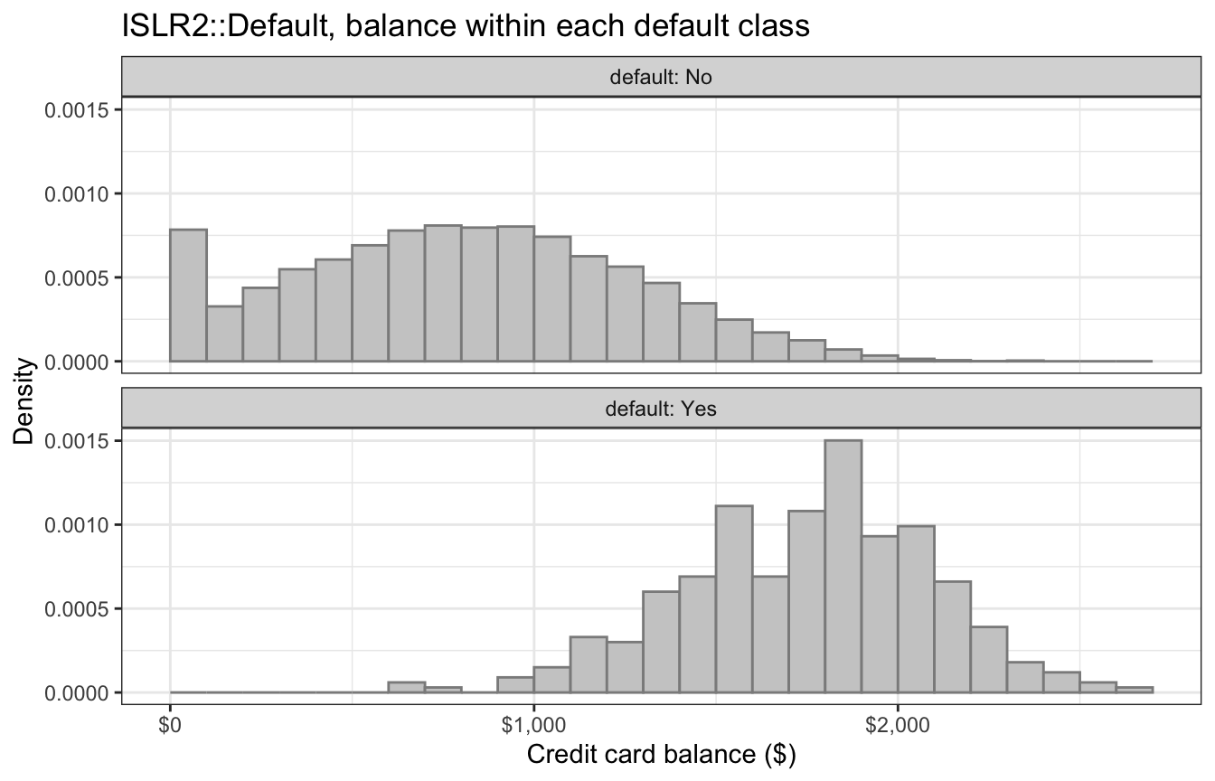
Each class’s balances form a single, roughly bell-shaped pile; the two piles are centered at different balances and have spreads of the same order. That suggests a model: describe each class’s balance by a Gaussian density with its own mean, the center of its pile, and one variance shared by both classes, the common width of the piles.

13.2.1 Gaussian class-conditional densities

With a single feature ($p = 1$) and observations indexed $i = 1, \ldots, n$, LDA assumes the statistical model

\[Y_i \stackrel{ind}{\sim} \text{Categorical}\left(\pi_1, \ldots, \pi_K\right), \qquad X_i \mid Y_i = k \stackrel{ind}{\sim} N\left(\mu_k, \sigma^2\right), \qquad i = 1, \ldots, n,\]

where

$Y_i$ is the class of observation $i$ and $X_i$ its feature value, both random, with observed values $y_i$ and $x_i$,
$\text{Categorical}\left(\pi_1, \ldots, \pi_K\right)$ is the distribution on the classes $\{1, \ldots, K\}$ with $P(Y_i = k) = \pi_k$,
$\stackrel{ind}{\sim}$ means independent over $i$: the $Y_i$ are independent, and given $Y_1, \ldots, Y_n$ the $X_i$ are independent, each depending only on its own class $Y_i$,
$\mu_k = E[X_i \mid Y_i = k]$ is the mean of the feature in class $k$, and
$\sigma^2 = Var[X_i \mid Y_i = k]$ is the variance of the feature, the same in every class.

A new observation $(X, Y)$, the one to be classified, follows the same model, so $\pi_k = P(Y = k)$ and $f_k$ is the density of $X$ given $Y = k$, as in Bayes’ theorem above. The class-conditional density is therefore the normal density

\[f_k(x) = \frac{1}{\sqrt{2\pi}\,\sigma} \exp\left[-\frac{(x - \mu_k)^2}{2\sigma^2}\right],\]

where $\pi$ without a subscript is the constant $3.14159\ldots$, unrelated to the prior probabilities $\pi_k$.

The classes differ only in where their densities are centered. For the credit card customers, $\mu_k$ is the center of class $k$’s pile of balances in the histograms above, and $\sigma$ is the width the two piles share.

13.2.2 Parameter estimation

The parameters $\pi_k$, $\mu_k$, and $\sigma^2$ are estimated from the observed training data $(x_1, y_1), \ldots, (x_n, y_n)$, here with $x_i$ the scalar feature value of observation $i$:

\[\hat\pi_k = \frac{n_k}{n}, \qquad \hat\mu_k = \frac{1}{n_k}\sum_{i:\, y_i = k} x_i, \qquad \hat\sigma^2 = \frac{1}{n - K}\sum_{k=1}^K \sum_{i:\, y_i = k}\left(x_i - \hat\mu_k\right)^2,\]

where

$n_k$ is the number of training observations in class $k$, so $\sum_k n_k = n$,
$\sum_{i:\, y_i = k}$ sums over the training observations in class $k$, and
$\hat\sigma^2$ is the pooled variance: squared deviations from each observation’s own class mean, summed over all classes and divided by $n - K$.

$\hat\pi_k$ and $\hat\mu_k$ are maximum likelihood estimates; $\hat\sigma^2$ is the maximum likelihood estimate rescaled by $n/(n - K)$ to make it unbiased. Under the generative model the joint density of observation $i$ is $P(Y_i = y_i)\, f_{y_i}(x_i) = \pi_{y_i} f_{y_i}(x_i)$, and the independence over $i$ in the model makes the likelihood the product of these densities, so the log-likelihood is

\[\ell(\pi_1, \ldots, \pi_K, \mu_1, \ldots, \mu_K, \sigma^2) = \sum_{k=1}^K n_k \log \pi_k \;+\; \sum_{k=1}^K \sum_{i:\, y_i = k}\left[-\frac{1}{2}\log\left(2\pi\sigma^2\right) - \frac{(x_i - \mu_k)^2}{2\sigma^2}\right].\]

The first sum involves only the priors; maximizing it subject to $\sum_k \pi_k = 1$ (with a Lagrange multiplier) gives $\hat\pi_k = n_k/n$. In the second, $\mu_k$ appears only in class $k$’s terms, so its maximizer is the class-$k$ sample mean. Setting the derivative with respect to $\sigma^2$ to zero gives the pooled sum of squares divided by $n$; dividing by $n - K$ instead, one degree of freedom per estimated mean, makes it unbiased, in the same way that $RSS/(n-2)$ replaced $RSS/n$ in simple linear regression. MASS::lda() uses $n - K$.

Logistic regression maximizes a different likelihood, the conditional one, $\prod_{i=1}^n p(x_i)^{y_i}\left[1 - p(x_i)\right]^{1 - y_i}$ (with $y_i$ coded $0/1$ as in the logistic regression lectures), which has no closed-form maximizer. LDA maximizes the joint likelihood of features and responses under a stronger assumption — Gaussian features with a shared variance — and every estimate is a sample proportion, mean, or variance.

MASS::lda() takes the same formula interface as glm(). Fitting default on balance prints three blocks: the prior probabilities, the group means, and the coefficients of linear discriminants.

balance_lda <- MASS::lda(default ~ balance, data = Default)
balance_lda

Call:
lda(default ~ balance, data = Default)

Prior probabilities of groups:
    No    Yes 
0.9667 0.0333 

Group means:
      balance
No   803.9438
Yes 1747.8217

Coefficients of linear discriminants:
                LD1
balance 0.002206916

Code

# Estimates of pi_k, mu_k, Sigma and the implied log posterior odds
# beta0 + x' beta of the second class, computed from the formulas above.
lda_by_hand <- function(X, y) {
  X <- as.matrix(X)
  classes <- levels(y)
  n <- nrow(X)
  K <- length(classes)
  pi_hat <- as.numeric(table(y)) / n
  mu_hat <- do.call(rbind, lapply(classes, function(k) {
    colMeans(X[y == k, , drop = FALSE])
  }))
  rownames(mu_hat) <- classes
  Sigma_hat <- Reduce(`+`, lapply(classes, function(k) {
    Z <- sweep(X[y == k, , drop = FALSE], 2, mu_hat[k, ])
    crossprod(Z)
  })) / (n - K)
  beta  <- solve(Sigma_hat, mu_hat[2, ] - mu_hat[1, ])
  beta0 <- log(pi_hat[2] / pi_hat[1]) -
    0.5 * (sum(mu_hat[2, ] * solve(Sigma_hat, mu_hat[2, ])) -
           sum(mu_hat[1, ] * solve(Sigma_hat, mu_hat[1, ])))
  list(pi = pi_hat, mu = mu_hat, Sigma = Sigma_hat,
       beta0 = beta0, beta = beta)
}

hand_1 <- lda_by_hand(Default["balance"], Default$default)
sigma_hat_1 <- sqrt(hand_1$Sigma[1, 1])

balance_grid <- tibble(balance = seq(0, 2800, length.out = 500))
gauss_curves <- tibble(default = factor(c("No", "Yes"))) |>
  mutate(mu = hand_1$mu[, 1]) |>
  cross_join(balance_grid) |>
  mutate(f = dnorm(balance, mu, sigma_hat_1))

gauss_plot <- balance_hist_plot +
  geom_line(data = gauss_curves, aes(y = f, color = default,
                                     linetype = default),
            linewidth = 0.9) +
  scale_color_manual(values = class_colors) +
  labs(color = "Default", linetype = "Default",
       title = expression(paste("Histograms with fitted ",
                                N(hat(mu)[k], hat(sigma)^2), " densities")))

The figure below draws each class’s fitted density $N\left(\hat\mu_k, \hat\sigma^2\right)$ over that class’s histogram from the start of this section.

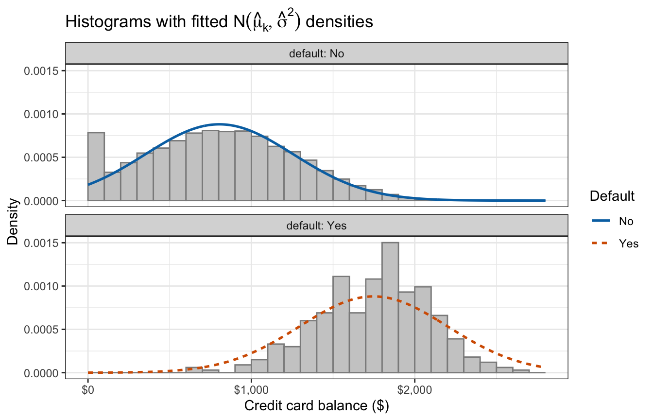
The prior probabilities are $\hat\pi_{\text{No}} = 0.9667$ and $\hat\pi_{\text{Yes}} = 0.0333$, the class proportions of the class summary table. The group means are $\hat\mu_{\text{No}} = 803.94$ and $\hat\mu_{\text{Yes}} = 1{,}747.82$ dollars, the mean balances of the same table. The pooled standard deviation is $\hat\sigma = 453.12$, between the two class-specific standard deviations.

In the figure, the fitted density for non-defaulters misses the spike at zero, and the one for defaulters, forced to share $\hat\sigma$ with the larger class, is wider than their histogram: the two departures from LDA’s assumptions that the histograms showed.

The coefficient of the linear discriminant, 0.002207, equals $1/\hat\sigma = 0.002207$: MASS::lda() reports the discriminant direction rescaled so that the printed linear combination, $\text{LD1} = \text{coefficient} \times \texttt{balance}$, has variance $1$ within each class, and with one feature the direction itself is just “larger balance points toward Yes.” This is Fisher’s scaling, described in the callout below.

Beyond this course

The “coefficients of linear discriminants” printed by MASS::lda() come from R. A. Fisher’s original formulation of discriminant analysis, which asks for the linear combination of features that maximizes the ratio of between-class to within-class variance and makes no Gaussian assumption. With $K$ classes that problem yields up to $K - 1$ discriminant directions, printed as LD1, LD2, …, and normalized to have unit within-class variance. With Gaussian classes and a shared covariance matrix, Fisher’s directions and the Bayes’-theorem discriminants of this lecture produce the same classifier.

For example,

LDA’s estimates have closed forms, and separation does not prevent them from existing, though a zero pooled variance still would. The previous lecture’s completely separated toy data, $x = 1, \ldots, 10$ with $y = 1$ exactly when $x > 5$, left logistic regression with no finite maximum likelihood estimate. MASS::lda() fits LDA to the same data:

toy <- tibble(x = 1:10, y = factor(as.numeric(x > 5)))
toy_lda <- MASS::lda(y ~ x, data = toy)
toy_lda$means

  x
0 3
1 8

The class means are 3 and 8 and the priors are equal, so LDA classifies by which class mean is closer: the boundary is their midpoint, 5.5.

13.2.3 Discriminant function

Since $p_k(x)$ is proportional to $\pi_k f_k(x)$ and the logarithm is increasing, the class with the largest posterior probability is also the class with the largest $\log\left[\pi_k f_k(x)\right]$. Expanding the square and collecting terms,

\[\log\left[\pi_k f_k(x)\right] = \log \pi_k - \frac{\mu_k^2}{2\sigma^2} + \frac{\mu_k}{\sigma^2}\, x - \log\left(\sqrt{2\pi}\,\sigma\right) - \frac{x^2}{2\sigma^2}.\]

The last two terms do not involve $k$ because $\sigma^2$ is shared, so they cannot change which class is largest. Dropping them gives the discriminant function

\[\delta_k(x) = \left(\log \pi_k - \frac{\mu_k^2}{2\sigma^2}\right) + \frac{\mu_k}{\sigma^2}\, x,\]

where

$\delta_k(x)$ is the discriminant value of class $k$ at feature value $x$,
$\log \pi_k - \mu_k^2/\left(2\sigma^2\right)$ is its intercept, the score at $x = 0$, and
$\mu_k/\sigma^2$ is its slope.

The dropped term $-x^2/\left(2\sigma^2\right)$ was the only one quadratic in $x$, so each $\delta_k$ is linear in $x$, with the same intercept-plus-slope form as a regression’s linear predictor. The classifier assigns an observation to the class with the largest $\delta_k(x)$. The slope $\mu_k/\sigma^2$ is not the coefficient of the linear discriminant printed by MASS::lda(), which is Fisher’s scaling of the discriminant direction.

Had the variances differed, with $\sigma_k^2$ the class-$k$ variance, the term $-\log\left(\sqrt{2\pi}\,\sigma_k\right)$ would differ between classes and stay in each intercept, and the term $-x^2/\left(2\sigma_k^2\right)$ would carry a different coefficient in each class, would not drop out, and would make each discriminant quadratic in $x$.

The terms dropped from $\log\left[\pi_k f_k(x)\right]$ to form $\delta_k(x)$ are the same in every class, so $e^{\delta_k(x)}$ is $\pi_k f_k(x)$ multiplied by a factor common to every class. That factor cancels from the ratio in Bayes’ theorem and the posterior probabilities can be recovered from the discriminant values alone:

\[p_k(x) = \frac{e^{\delta_k(x)}}{\sum_{l=1}^K e^{\delta_l(x)}}.\]

Code

delta_1 <- tibble(default = c("No", "Yes"),
                  intercept = log(hand_1$pi) -
                    hand_1$mu[, 1]^2 / (2 * sigma_hat_1^2),
                  slope = hand_1$mu[, 1] / sigma_hat_1^2)
delta_of <- function(k, col) delta_1[[col]][delta_1$default == k]

Substituting $\hat\pi_k$, $\hat\mu_k$, and $\hat\sigma^2$ for the credit card customers gives the estimated discriminants, with balance in dollars,

\[\hat\delta_{\text{No}}(x) = -1.608 + 0.003916\, x, \qquad \hat\delta_{\text{Yes}}(x) = -10.842 + 0.008513\, x.\]

The defaulters’ line starts far lower, because $\hat\pi_{\text{Yes}}$ is small and $\hat\mu_{\text{Yes}}$ large, and climbs 2.2 times as fast, because $\hat\mu_{\text{Yes}}$ is the larger mean.

13.2.4 Decision boundary

With $K = 2$ classes, $p_1(x) = 1 - p_2(x)$, and the log posterior odds of class $2$ are

\[\log\left[\frac{p_2(x)}{1 - p_2(x)}\right] = \delta_2(x) - \delta_1(x) = \underbrace{\log\frac{\pi_2}{\pi_1} - \frac{\mu_2^2 - \mu_1^2}{2\sigma^2}}_{\beta_0} + \underbrace{\frac{\mu_2 - \mu_1}{\sigma^2}}_{\beta_1}\, x.\]

The log-odds are linear in $x$, so LDA’s posterior probability has exactly the form of a simple logistic regression. The two methods differ in how they estimate $\beta_0$ and $\beta_1$, not in the shape of the curve they fit.

The decision boundary is the set of $x$ where the two classes are equally probable, $\delta_1(x) = \delta_2(x)$. Setting the log posterior odds to zero and solving,

\[x^* = \frac{\mu_1 + \mu_2}{2} + \frac{\sigma^2}{\mu_2 - \mu_1}\log\frac{\pi_1}{\pi_2},\]

where

$x^*$ is the feature value at which the classifier switches from one class to the other.

With equal prior probabilities the logarithm is zero and the boundary is the midpoint of the two means. Take $\mu_2 > \mu_1$. If class $2$ is the rarer class, $\pi_2 < \pi_1$, the logarithm is positive and the boundary moves to the right, toward $\mu_2$, and past it once $\sigma^2 \log(\pi_1/\pi_2)/(\mu_2 - \mu_1) > (\mu_2 - \mu_1)/2$: an observation must look more like a typical class-$2$ observation before the classifier assigns it to the rarer class. Since $\delta_1(x) = \delta_2(x)$ exactly where $\pi_1 f_1(x) = \pi_2 f_2(x)$, the boundary is also where the two prior-weighted densities cross.

Code

x_mid <- mean(hand_1$mu[, 1])
x_star_lda <- -hand_1$beta0 / hand_1$beta[1]

# Prior-weighted densities pi_k f_k(x) and discriminant functions delta_k(x)
# for the fitted means and pooled variance, under a given pair of priors.
weighted_curves <- function(priors) {
  tibble(default = factor(c("No", "Yes")), mu = hand_1$mu[, 1],
         prior = priors) |>
    cross_join(balance_grid) |>
    mutate(weighted = prior * dnorm(balance, mu, sigma_hat_1),
           delta = (log(prior) - mu^2 / (2 * sigma_hat_1^2)) +
                   mu / sigma_hat_1^2 * balance)
}

weighted_plot <- function(priors, boundary, title, y_label) {
  ggplot(weighted_curves(priors),
         aes(x = balance, y = weighted, color = default, linetype = default)) +
    geom_line(linewidth = 0.9) +
    geom_vline(xintercept = boundary, linetype = "dotted") +
    scale_color_manual(values = class_colors) +
    scale_x_continuous(labels = dollar_labels) +
    labs(x = "Credit card balance ($)",
         y = y_label,
         color = "Default", linetype = "Default", title = title)
}

equal_priors_plot <- weighted_plot(
  c(0.5, 0.5), x_mid,
  expression(paste("Equal priors, ", pi[No] == pi[Yes], " = 0.5")),
  expression(pi[k] * hat(f)[k](x)))
estimated_priors_plot <- weighted_plot(
  hand_1$pi, x_star_lda,
  bquote(paste("Estimated priors, ",
               hat(pi)[Yes] == .(sprintf("%.4f", hand_1$pi[2])))),
  expression(hat(pi)[k] * hat(f)[k](x)))

delta_default_plot <- ggplot(weighted_curves(hand_1$pi),
                             aes(x = balance, y = delta,
                                 color = default, linetype = default)) +
  geom_line(linewidth = 0.9) +
  geom_vline(xintercept = x_star_lda, linetype = "dotted") +
  scale_color_manual(values = class_colors) +
  scale_x_continuous(labels = dollar_labels) +
  labs(x = "Credit card balance ($)", y = expression(hat(delta)[k](x)),
       color = "Default", linetype = "Default",
       title = "Estimated discriminant functions, estimated priors")

For the credit card fit, the first tab below plots the prior-weighted fitted densities with equal priors, a counterfactual in which defaulting is as common as not, and the second with the estimated priors. The third plots the two estimated discriminant functions. In every tab a dotted line marks that tab’s decision boundary.

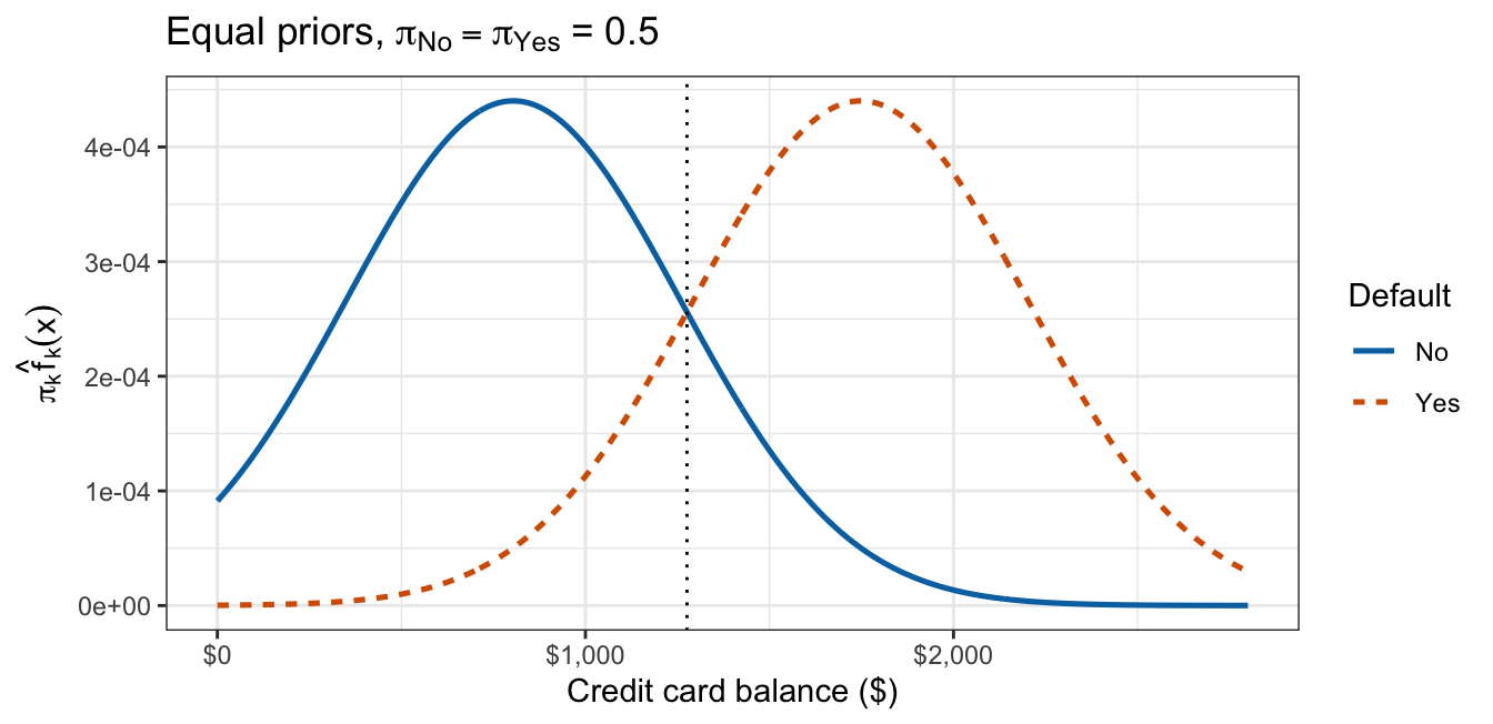
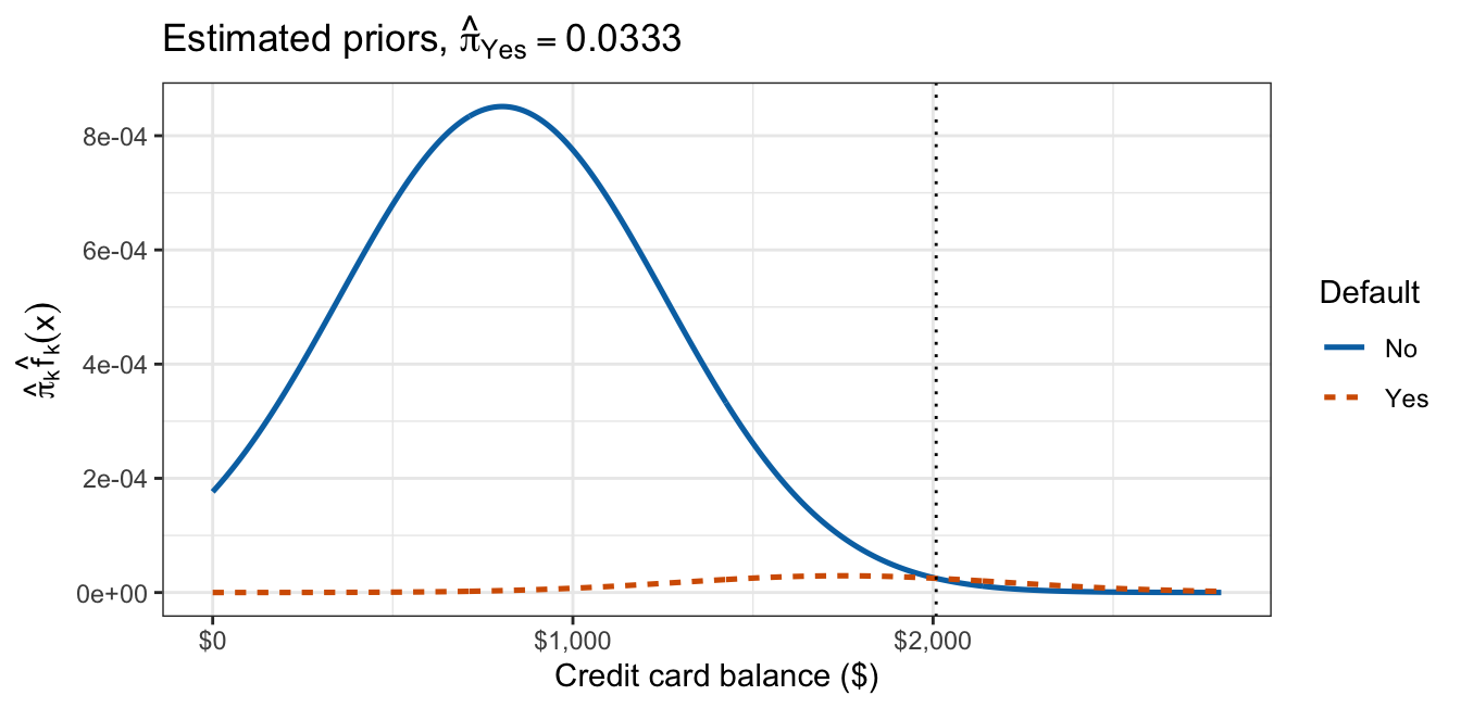
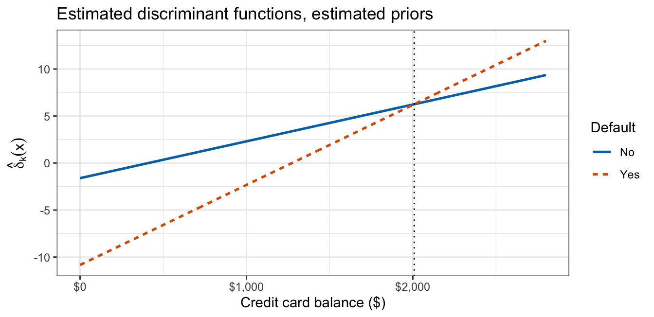
With equal priors the two curves are the same height and cross at the midpoint of the class means, $1,276. With the estimated priors the defaulter curve shrinks to a small bump that rises above the non-defaulter curve only past $\hat x^* = \$2{,}009$, deep in the non-defaulters’ right tail. In the boundary formula that shift is the prior term $\hat\sigma^2\log\left(\hat\pi_{\text{No}}/\hat\pi_{\text{Yes}}\right)/\left(\hat\mu_{\text{Yes}} - \hat\mu_{\text{No}}\right)$, which adds $733 because $\hat\pi_{\text{Yes}}$ is so small. The boundary lies beyond $\hat\mu_{\text{Yes}} = \$1{,}748$, so even a customer with the defaulters’ average balance is classified No. The discriminant functions are two straight lines crossing at the same balance. A linear discriminant function for each class, with the boundary where two of them are equal, is the “linear” in linear discriminant analysis.

13.2.5 Simple logistic regression comparison

Because the log posterior odds are linear in $x$, LDA’s fit can be set beside the simple logistic regression of the same customers on the log-odds scale.

Code

balance_glm <- glm(default ~ balance, data = Default, family = "binomial")
b_glm_1     <- coef(balance_glm)
x_star_glm  <- -b_glm_1[1] / b_glm_1[2]

post_1 <- predict(balance_lda)$posterior[, "Yes"]
max_diff_1 <- max(abs(post_1 - plogis(hand_1$beta0 +
                                       hand_1$beta[1] * Default$balance)))

coef_table_1 <- tibble(
  term = c("Intercept $\\hat\\beta_0$", "`balance` $\\hat\\beta_1$"),
  lda = c(hand_1$beta0, hand_1$beta[1]),
  glm = unname(b_glm_1)
) |>
  mutate(across(c(lda, glm), \(v) sprintf("%.6f", v))) |>
  knitr::kable(col.names = c("Coefficient", "LDA", "Logistic regression"),
               align = "lcc")

posterior_curves <- balance_grid |>
  mutate(LDA = plogis(hand_1$beta0 + hand_1$beta[1] * balance),
         `Logistic regression` = predict(balance_glm,
                                         newdata = balance_grid,
                                         type = "response")) |>
  pivot_longer(-balance, names_to = "model", values_to = "p_hat")

posterior_default_plot <- ggplot(posterior_curves,
                                 aes(x = balance, y = p_hat)) +
  geom_point(data = Default, aes(y = default_jit), alpha = 0.08,
             size = 0.7) +
  geom_hline(yintercept = 0.5, color = "grey60") +
  geom_line(aes(color = model, linetype = model), linewidth = 0.9) +
  scale_color_manual(values = model_colors) +
  scale_y_continuous(breaks = c(0, 0.5, 1)) +
  scale_x_continuous(labels = dollar_labels) +
  labs(x = "Credit card balance ($)", y = "P(default = Yes)",
       color = "Model", linetype = "Model",
       title = "Posterior probability of default")

The table gives LDA’s $\hat\beta_0$ and $\hat\beta_1$, from the estimates above, beside the simple logistic regression’s coefficients. The figure plots both models’ probability of default against balance, with each customer’s jittered outcome and a grey line at $0.5$.

Coefficient	LDA	Logistic regression
Intercept $\hat\beta_0$	-9.233739	-10.651331
`balance` $\hat\beta_1$	0.004597	0.005499

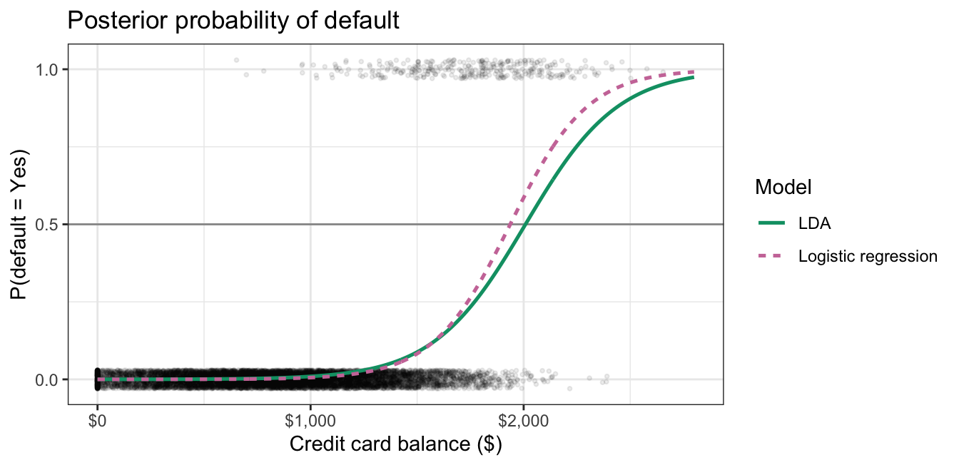
The intercept $\hat\beta_0 = -9.234$ is LDA’s estimated log posterior odds of default for a customer carrying no balance, a posterior probability of 0.000098. Each additional $100 of balance adds 0.460 to the log posterior odds, against 0.550 in the logistic regression. Applying the logistic function to $\hat\beta_0 + \hat\beta_1 x$ reproduces the posterior probabilities returned by predict() to within $1 \times 10^{-14}$.

The LDA curve is a logistic curve, slightly flatter than the logistic regression fit, and it crosses $0.5$ a little further right, at $2,009 against $1,937. Logistic regression has no priors or class means; its boundary is high because defaults are rare among customers at all but the largest balances, so its fitted probability reaches $0.5$ only there.

13.3 Multiple-feature LDA

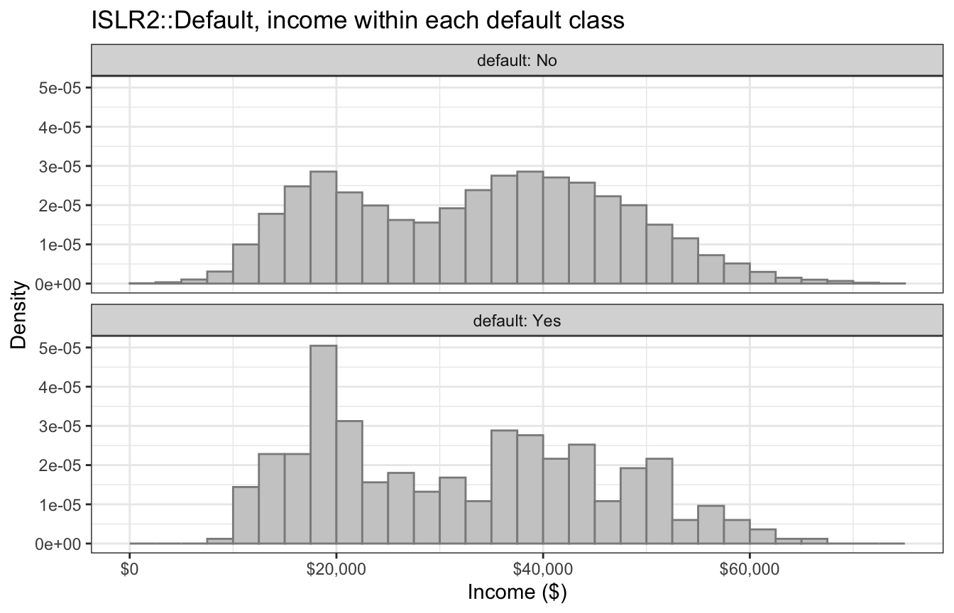
A second feature turns each customer into a point. The first tab below plots income against credit card balance for every customer, with defaulters and non-defaulters distinguished by color and shape; the second shows income within each default class, one panel per class, on the density scale.

Code

# Defaulters are drawn last so they are not hidden under non-defaulters.
scatter_base <- ggplot(arrange(Default, default),
                       aes(x = balance, y = income)) +
  geom_point(aes(color = default, shape = default), alpha = 0.35,
             size = 0.8) +
  scale_color_manual(values = class_colors) +
  scale_shape_manual(values = c(16, 17)) +
  guides(color = guide_legend(override.aes = list(alpha = 1, size = 2))) +
  scale_x_continuous(labels = dollar_labels) +
  scale_y_continuous(labels = dollar_labels) +
  labs(x = "Credit card balance ($)", y = "Income ($)", color = "Default",
       shape = "Default")

eda_scatter <- scatter_base +
  labs(title = "ISLR2::Default, income against balance")

income_hist_plot <- ggplot(Default, aes(x = income)) +
  geom_histogram(aes(y = after_stat(density)), binwidth = 2500,
                 boundary = 0, fill = "grey80", color = "grey55") +
  facet_wrap(~ default, ncol = 1, labeller = label_both) +
  scale_x_continuous(labels = dollar_labels) +
  labs(x = "Income ($)", y = "Density",
       title = "ISLR2::Default, income within each default class")

within_cor <- Default |>
  group_by(default) |>
  summarize(r = cor(balance, income), mean_income = mean(income),
            .groups = "drop")
within_of <- function(k, col) within_cor[[col]][within_cor$default == k]

income_by_student <- Default |>
  group_by(student) |>
  summarize(median_income = median(income), .groups = "drop")
student_income <- function(s) {
  income_by_student$median_income[income_by_student$student == s]
}

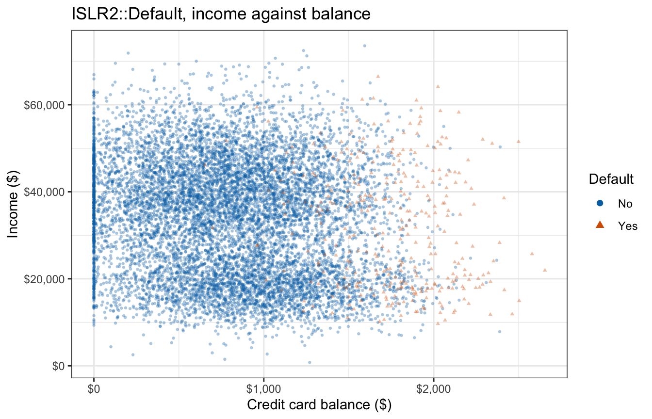
Each class forms a broad cloud, and the two clouds overlap heavily: defaulters sit at larger balances, across nearly the whole range of income. Within each class balance and income are weakly negatively correlated, $r = -0.155$ among non-defaulters and $r = -0.166$ among defaulters, so a description of each class’s cloud needs a center and a spread for each feature and the correlation between them. The two classes’ mean incomes are close, $32,089 for defaulters against $33,566.

The two classes’ income histograms look alike, and each is bimodal. The lower mode is mostly students: in these data students’ median income is $17,994, against $39,893 for non-students. No Gaussian density has two modes, so income strains LDA’s assumptions just as balance did.

The clouds suggest the multivariate version of the one-feature model: describe each class’s features by a multivariate Gaussian density with its own mean vector, the center of its cloud, and a covariance matrix shared by both classes, which gives the clouds one common spread and tilt.

13.3.1 Multivariate Gaussian densities

With $p > 1$ features, the features of observation $i$ form a random column vector $X_i = (X_{i1}, \ldots, X_{ip})^\top$, and $x$ is a $p$-vector value it takes. A value $x$ holds the same kind of entries as a row of the model matrix $\mathbf{X}$ but without the leading $1$, and it is a column because it is the argument of a multivariate density. LDA assumes the statistical model

\[Y_i \stackrel{ind}{\sim} \text{Categorical}\left(\pi_1, \ldots, \pi_K\right), \qquad X_i \mid Y_i = k \stackrel{ind}{\sim} N_p\left(\mu_k, \Sigma\right), \qquad i = 1, \ldots, n,\]

where

$Y_i$, $\text{Categorical}\left(\pi_1, \ldots, \pi_K\right)$, and $\stackrel{ind}{\sim}$ are as in the one-feature model, so the observations are independent while the $p$ features within one observation may be correlated,
$N_p$ is the $p$-dimensional multivariate normal distribution,
$\mu_k = E[X_i \mid Y_i = k] = (\mu_{k1}, \ldots, \mu_{kp})^\top$ is the $p$-vector of feature means in class $k$, and
$\Sigma = Cov[X_i \mid Y_i = k]$ is the $p \times p$ covariance matrix of the features, the same in every class, with feature variances on its diagonal and covariances between pairs of features off it; it is symmetric and positive definite.

The class-conditional density is therefore the multivariate normal density

\[f_k(x) = \frac{1}{(2\pi)^{p/2}\,|\Sigma|^{1/2}} \exp\left[-\frac{1}{2}\left(x - \mu_k\right)^\top \Sigma^{-1} \left(x - \mu_k\right)\right],\]

where $|\Sigma|$ is the determinant of $\Sigma$.

Each class’s density has contours that are nested ellipses centered at $\mu_k$. Sharing $\Sigma$ means every class’s ellipses have the same shape and orientation and differ only in their center. For the credit card customers, $\mu_k$ is the center of class $k$’s cloud in the scatterplot above, and $\Sigma$ gives the two clouds one common spread and tilt.

13.3.2 Pooled covariance estimate

The estimates generalize directly. The priors are still $\hat\pi_k = n_k/n$, and with $x_i = (x_{i1}, \ldots, x_{ip})^\top$ now the observed value of $X_i$, the $p$-vector of feature values for observation $i$ (again without the leading $1$),

\[\hat\mu_k = \frac{1}{n_k}\sum_{i:\, y_i = k} x_i, \qquad \hat\Sigma = \frac{1}{n - K}\sum_{k=1}^K \sum_{i:\, y_i = k}\left(x_i - \hat\mu_k\right)\left(x_i - \hat\mu_k\right)^\top,\]

where

$\hat\mu_k$ is the vector of class-$k$ sample means, one per feature, and
$\hat\Sigma$ is the pooled covariance matrix, the sum of each class’s matrix of cross-products of deviations from its own mean, divided by $n - K$; as in one dimension, it is the maximum likelihood estimate rescaled by $n/(n - K)$ to make it unbiased.

Adding income to the formula fits the $p = 2$ model to the credit card customers:

additive_lda <- MASS::lda(default ~ balance + income, data = Default)
additive_lda

Call:
lda(default ~ balance + income, data = Default)

Prior probabilities of groups:
    No    Yes 
0.9667 0.0333 

Group means:
      balance   income
No   803.9438 33566.17
Yes 1747.8217 32089.15

Coefficients of linear discriminants:
                 LD1
balance 2.230835e-03
income  7.793355e-06

Code

X2 <- as.matrix(Default[c("balance", "income")])
hand_2 <- lda_by_hand(X2, Default$default)

scaling_ratio <- additive_lda$scaling[, 1] / hand_2$beta
sd_within <- sqrt(diag(hand_2$Sigma))
cor_within <- hand_2$Sigma[1, 2] / prod(sd_within)

post_lda_2 <- predict(additive_lda)$posterior[, "Yes"]
max_diff_2 <- max(abs(post_lda_2 -
                      plogis(hand_2$beta0 + drop(X2 %*% hand_2$beta))))

The prior probabilities are unchanged, since they do not depend on the features. The group means now form a vector for each class: the balance column repeats the one-feature means, and the income column holds the class mean incomes. The pooled covariance matrix $\hat\Sigma$ has within-class standard deviations of $453 for balance and $13,335 for income and a within-class correlation of $-0.155$, a pooled version of the two correlations quoted with the scatterplot.

13.3.3 Matrix-form discriminant

The derivation follows the one-feature case. Because $\Sigma^{-1}$ is symmetric, the scalar $\mu_k^\top \Sigma^{-1} x$ equals its own transpose $x^\top \Sigma^{-1} \mu_k$, and the quadratic form expands to

\[\left(x - \mu_k\right)^\top \Sigma^{-1} \left(x - \mu_k\right) = x^\top \Sigma^{-1} x - 2\, x^\top \Sigma^{-1} \mu_k + \mu_k^\top \Sigma^{-1} \mu_k.\]

Then, collecting terms in the same order as before,

\[\log\left[\pi_k f_k(x)\right] = \log \pi_k - \frac{1}{2}\mu_k^\top \Sigma^{-1} \mu_k + x^\top \Sigma^{-1} \mu_k - \frac{p}{2}\log(2\pi) - \frac{1}{2}\log|\Sigma| - \frac{1}{2}x^\top \Sigma^{-1} x.\]

The last three terms do not involve $k$: the first is a constant, and the other two because $\Sigma$ is shared. Dropping them gives

\[\delta_k(x) = \left(\log \pi_k - \frac{1}{2}\mu_k^\top \Sigma^{-1} \mu_k\right) + x^\top \Sigma^{-1} \mu_k,\]

where

$\log \pi_k - \frac{1}{2}\mu_k^\top \Sigma^{-1} \mu_k$ is the intercept of class $k$’s discriminant, and
$\Sigma^{-1}\mu_k$ is its $p$-vector of slopes, one per feature.

The dropped term $-\frac{1}{2}x^\top \Sigma^{-1} x$ was the only one quadratic in $x$, so the discriminant is linear in $x$ and reduces to the one-feature discriminant when $\Sigma = \sigma^2$. As before, the classifier assigns the class with the largest $\delta_k(x)$, and $p_k(x) = e^{\delta_k(x)} / \sum_l e^{\delta_l(x)}$.

Code

Sigma2_inv <- solve(hand_2$Sigma)
# Each class's estimated discriminant: intercept and slopes Sigma^{-1} mu_k.
delta_row_2 <- function(k) {
  slopes <- drop(Sigma2_inv %*% hand_2$mu[k, ])
  tibble(default = k,
         intercept = log(hand_2$pi[rownames(hand_2$mu) == k]) -
           0.5 * sum(hand_2$mu[k, ] * slopes),
         balance = slopes[1], income = 1000 * slopes[2])
}
delta_table_2 <- map(c("No", "Yes"), delta_row_2) |> list_rbind()
delta_kable_2 <- delta_table_2 |>
  mutate(intercept = sprintf("%.3f", intercept),
         balance = sprintf("%.6f", balance),
         income = sprintf("%.6f", income)) |>
  knitr::kable(col.names = c("Default", "Intercept", "`balance` slope",
                             "`income` slope, per \\$1,000"),
               align = "lccc")

For the credit card fit, the table gives each class’s estimated discriminant, $\hat\delta_k(x)$, with income slopes per $1,000 of income.

Default	Intercept	`balance` slope	`income` slope, per $1,000
No	-5.603	0.004895	0.214577
Yes	-15.467	0.009567	0.230897

As in one dimension, the defaulters’ discriminant starts far lower and climbs faster in balance. Its income slope is also the larger of the two, so at a fixed balance a higher income moves the comparison slightly toward Yes.

13.3.4 Linear decision boundary

With $K = 2$, subtracting the two discriminants gives the log posterior odds of class $2$,

\[\log\left[\frac{p_2(x)}{1 - p_2(x)}\right] = \delta_2(x) - \delta_1(x) = \beta_0 + x^\top\beta,\]

where

$\beta = \Sigma^{-1}(\mu_2 - \mu_1)$ is a $p$-vector of slopes, one per feature, with no intercept entry, and
$\beta_0 = \log(\pi_2/\pi_1) - \frac{1}{2}\left(\mu_2^\top \Sigma^{-1} \mu_2 - \mu_1^\top \Sigma^{-1} \mu_1\right)$ is the intercept.

This is again the form of a multiple logistic regression with $p$ features. The decision boundary $\{x : \beta_0 + x^\top\beta = 0\}$ is a hyperplane in the $p$-dimensional feature space — a line when $p = 2$.

The slopes are $\Sigma^{-1}(\mu_2 - \mu_1)$, not $\mu_2 - \mu_1$, so the boundary is generally not perpendicular to the segment joining the two means: $\Sigma^{-1}$ tilts it according to how the features covary. With equal priors it still passes through the midpoint $(\mu_1 + \mu_2)/2$, since substituting that point gives $\frac{1}{2}\left(\mu_1 + \mu_2\right)^\top\Sigma^{-1}\left(\mu_2 - \mu_1\right) = \frac{1}{2}\left(\mu_2^\top \Sigma^{-1} \mu_2 - \mu_1^\top \Sigma^{-1} \mu_1\right)$. The boundary is where $\pi_1 f_1(x) = \pi_2 f_2(x)$, so it passes through every point where a contour of $\pi_1 f_1$ crosses the contour of $\pi_2 f_2$ of the same height.

Code

mu_No  <- hand_2$mu["No", ]
mu_Yes <- hand_2$mu["Yes", ]
beta_2 <- hand_2$beta
f_peak_2 <- 1 / (2 * pi * sqrt(det(hand_2$Sigma)))
dens_2 <- function(b, i, mu) {
  d <- cbind(b - mu[1], i - mu[2])
  f_peak_2 * exp(-rowSums((d %*% Sigma2_inv) * d) / 2)
}

window_2 <- list(balance = c(0, 2700), income = c(0, 75000))
grid_2 <- expand_grid(balance = seq(0, 2700, length.out = 240),
                      income = seq(0, 75000, length.out = 220)) |>
  mutate(f_No = dens_2(balance, income, mu_No),
         f_Yes = dens_2(balance, income, mu_Yes))

# Long grid of pi_k * f_k(x); prior weights of 1 give the unweighted f_k.
weighted_grid_2 <- function(p) {
  grid_2 |>
    transmute(balance, income, No = p[1] * f_No, Yes = p[2] * f_Yes) |>
    pivot_longer(c(No, Yes), names_to = "default", values_to = "density")
}

# Fitted densities: contours where (x - mu_k)' Sigma^{-1} (x - mu_k) is 1 and
# 4. Prior-weighted
# densities: the same three heights, as fractions of the peak of f_k, in both
# prior tabs.
density_levels_2  <- f_peak_2 * exp(-c(1, 2)^2 / 2)
weighted_levels_2 <- f_peak_2 * c(0.01, 0.02, 0.03)

beta0_2 <- function(p) {
  log(p[2] / p[1]) -
    0.5 * (sum(mu_Yes * (Sigma2_inv %*% mu_Yes)) -
           sum(mu_No * (Sigma2_inv %*% mu_No)))
}
# beta0 + beta1 balance + beta2 income = 0 => income = intercept + slope balance
line_2 <- function(p) {
  c(intercept = unname(-beta0_2(p) / beta_2[2]),
    slope = unname(-beta_2[1] / beta_2[2]))
}

# Where the same-height contours of the two classes cross: where the boundary
# line, on which pi_1 f_1 = pi_2 f_2, meets the class-1 contour at that height.
# Along the line x = p0 + s u, log(pi_1 f_1(x)) is quadratic in s. Only
# crossings inside the plotted window are kept.
crossings_2 <- function(p, levels) {
  p0 <- -beta0_2(p) * beta_2 / sum(beta_2^2)
  u  <- c(beta_2[2], -beta_2[1])
  d0 <- p0 - mu_No
  a  <- 0.5 * sum(u * (Sigma2_inv %*% u))
  b  <- sum(u * (Sigma2_inv %*% d0))
  map(levels, \(L) {
    c0 <- 0.5 * sum(d0 * (Sigma2_inv %*% d0)) - log(p[1] * f_peak_2 / L)
    disc <- b^2 - 4 * a * c0
    if (disc < 0) return(NULL)
    s <- (-b + c(-1, 1) * sqrt(disc)) / (2 * a)
    tibble(balance = p0[1] + s * u[1], income = p0[2] + s * u[2])
  }) |>
    list_rbind() |>
    filter(between(balance, window_2$balance[1], window_2$balance[2]),
           between(income, window_2$income[1], window_2$income[2]))
}

means_2 <- tibble(balance = c(mu_No[1], mu_Yes[1]),
                  income = c(mu_No[2], mu_Yes[2]))

contour_plot_2 <- function(p, levels) {
  ggplot(weighted_grid_2(p), aes(x = balance, y = income)) +
    geom_point(data = Default, aes(color = default, shape = default),
               alpha = 0.12, size = 0.6) +
    geom_contour(aes(z = density, color = default, linetype = default),
                 breaks = levels, linewidth = 0.8) +
    geom_line(data = means_2, color = "grey40", linewidth = 0.5) +
    geom_point(data = means_2, shape = 4, size = 4, stroke = 1.5) +
    scale_color_manual(values = class_colors) +
    scale_shape_manual(values = c(16, 17)) +
    scale_x_continuous(labels = dollar_labels) +
    scale_y_continuous(labels = dollar_labels) +
    coord_cartesian(xlim = window_2$balance, ylim = window_2$income) +
    guides(color = guide_legend(override.aes = list(alpha = 1))) +
    labs(x = "Credit card balance ($)", y = "Income ($)", color = "Default",
         shape = "Default", linetype = "Default")
}
# The boundary uses "longdash", distinct from both class-contour linetypes.
boundary_line_2 <- function(p, ...) {
  l <- line_2(p)
  geom_abline(intercept = l["intercept"], slope = l["slope"], ...)
}
crossing_points_2 <- function(p) {
  geom_point(data = crossings_2(p, weighted_levels_2),
             aes(x = balance, y = income), inherit.aes = FALSE,
             shape = 21, size = 3, stroke = 1, fill = "white", color = "black")
}

contour_densities_2 <- contour_plot_2(c(1, 1), density_levels_2) +
  labs(title = expression(paste("Contours of ", hat(f)[k](x))))
contour_equal_2 <- contour_plot_2(c(0.5, 0.5), weighted_levels_2) +
  boundary_line_2(c(0.5, 0.5), linewidth = 1, linetype = "longdash") +
  crossing_points_2(c(0.5, 0.5)) +
  labs(title = expression(paste("Contours of ", pi[k] * hat(f)[k](x), "; ",
                                pi[No] == pi[Yes], " = 0.5")))
contour_estimated_2 <- contour_plot_2(hand_2$pi, weighted_levels_2) +
  boundary_line_2(c(0.5, 0.5), linewidth = 0.6, color = "grey50",
                  linetype = "dotted") +
  boundary_line_2(hand_2$pi, linewidth = 1, linetype = "longdash") +
  crossing_points_2(hand_2$pi) +
  labs(title = bquote(paste("Contours of ", hat(pi)[k] * hat(f)[k](x), "; ",
                            hat(pi)[Yes] == .(sprintf("%.4f", hand_2$pi[2])))))

# Read as a balance threshold at a given income, and over the whole observed
# range of income; and the change in the log posterior odds per standard
# deviation of each feature.
threshold_at <- function(b0, b1, b2, inc) -(b0 + b2 * inc) / b1
x_star_lda_range <- threshold_at(hand_2$beta0, hand_2$beta[1],
                                 hand_2$beta[2], range(Default$income))
per_sd_lda <- hand_2$beta * c(sd(Default$balance), sd(Default$income))
yes_peak_share <- hand_2$pi[2]

For the credit card fit, each tab below draws faint customer points, the two estimated class means (crosses) joined by a grey segment, and contours: the first tab draws two contours of each class’s fitted density $\hat f_k$, the ellipses on which $\left(x - \hat\mu_k\right)^\top \hat\Sigma^{-1} \left(x - \hat\mu_k\right)$ equals $1$ and $4$, and the second and third draw contours of the prior-weighted densities at the same three heights, $\pi_k \hat f_k$ with equal priors and $\hat\pi_k \hat f_k$ with the estimated priors, together with that tab’s decision boundary (long dashes). Open circles mark where a non-defaulter contour crosses the defaulter contour of the same height, and the dotted line in the third tab is the equal-prior boundary.

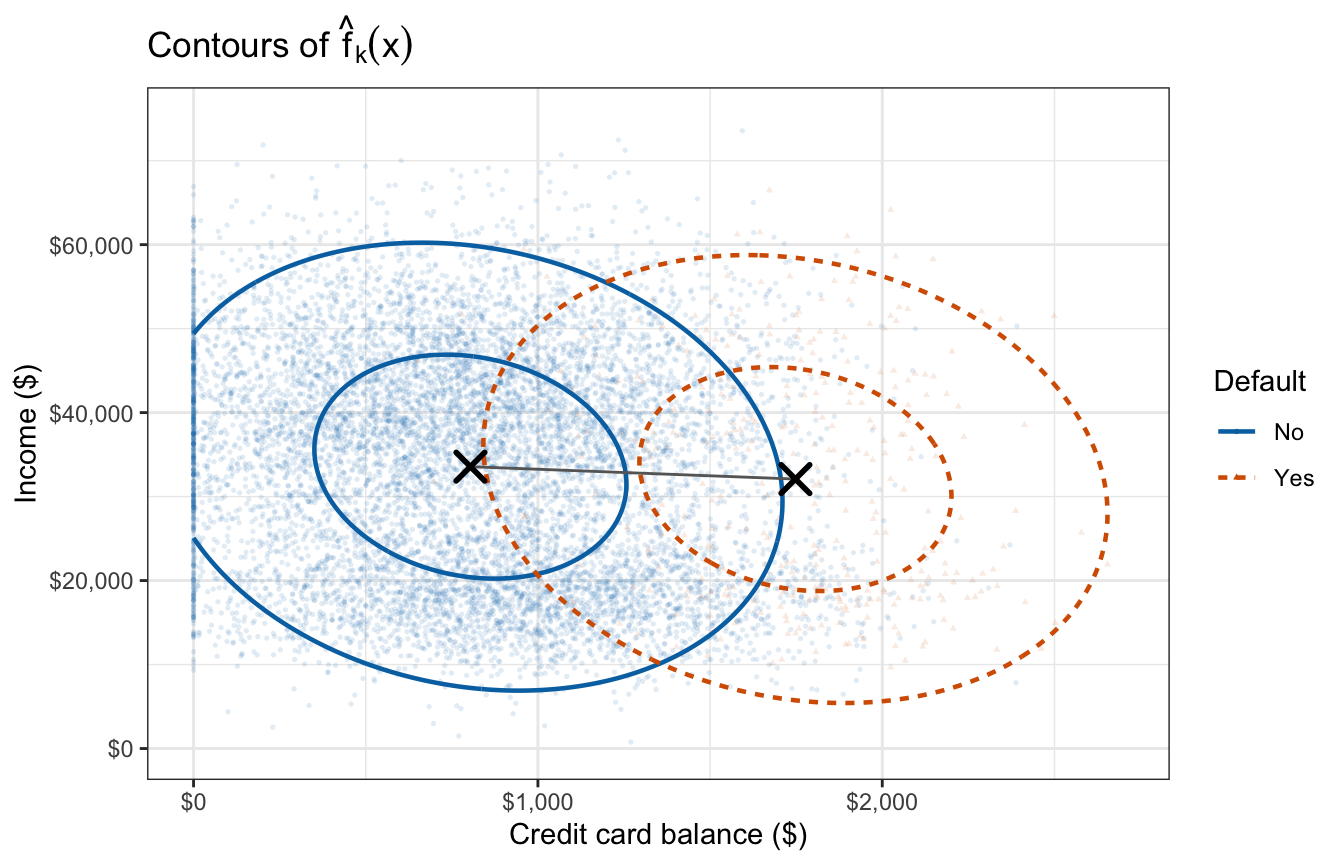
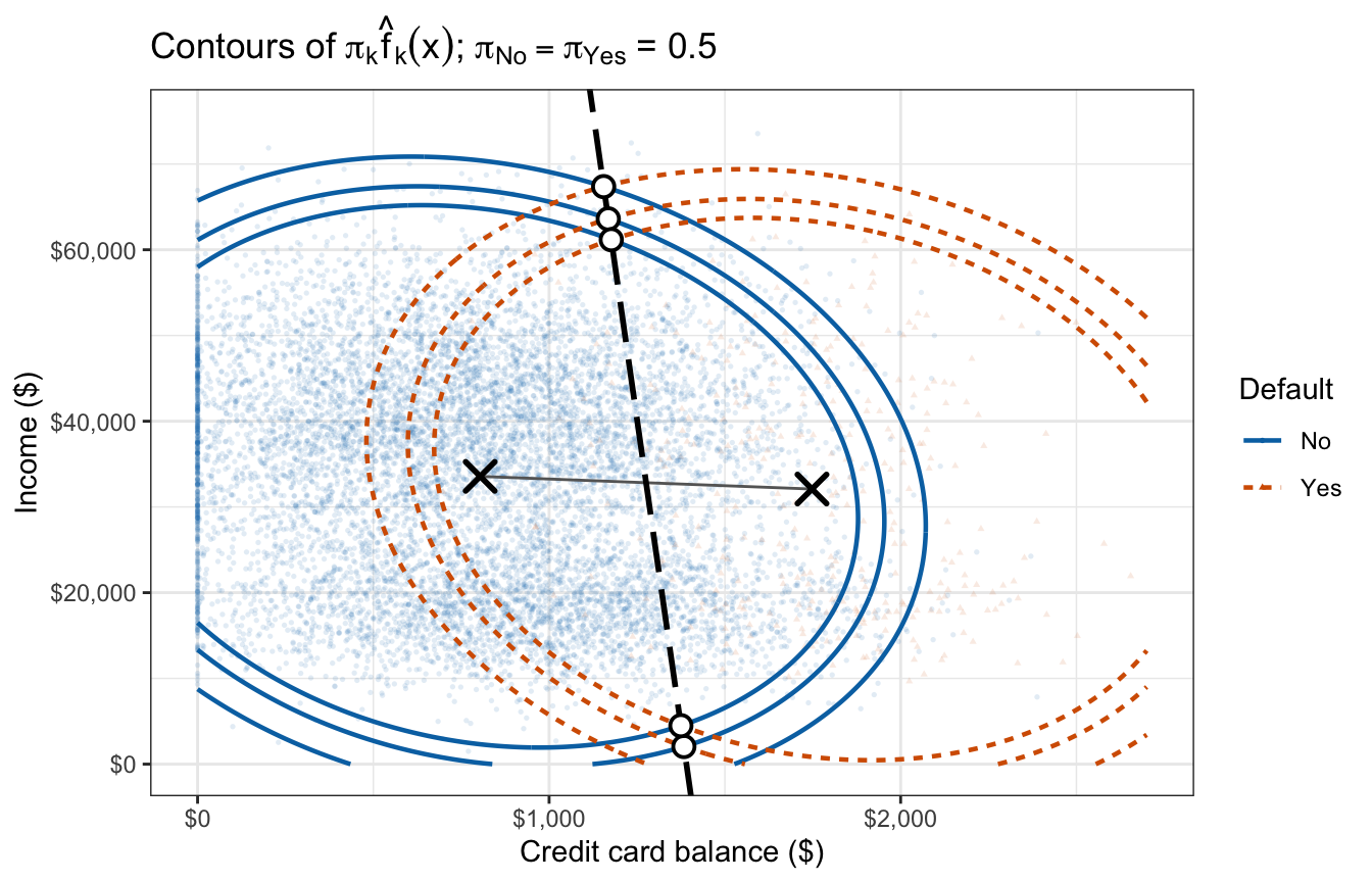
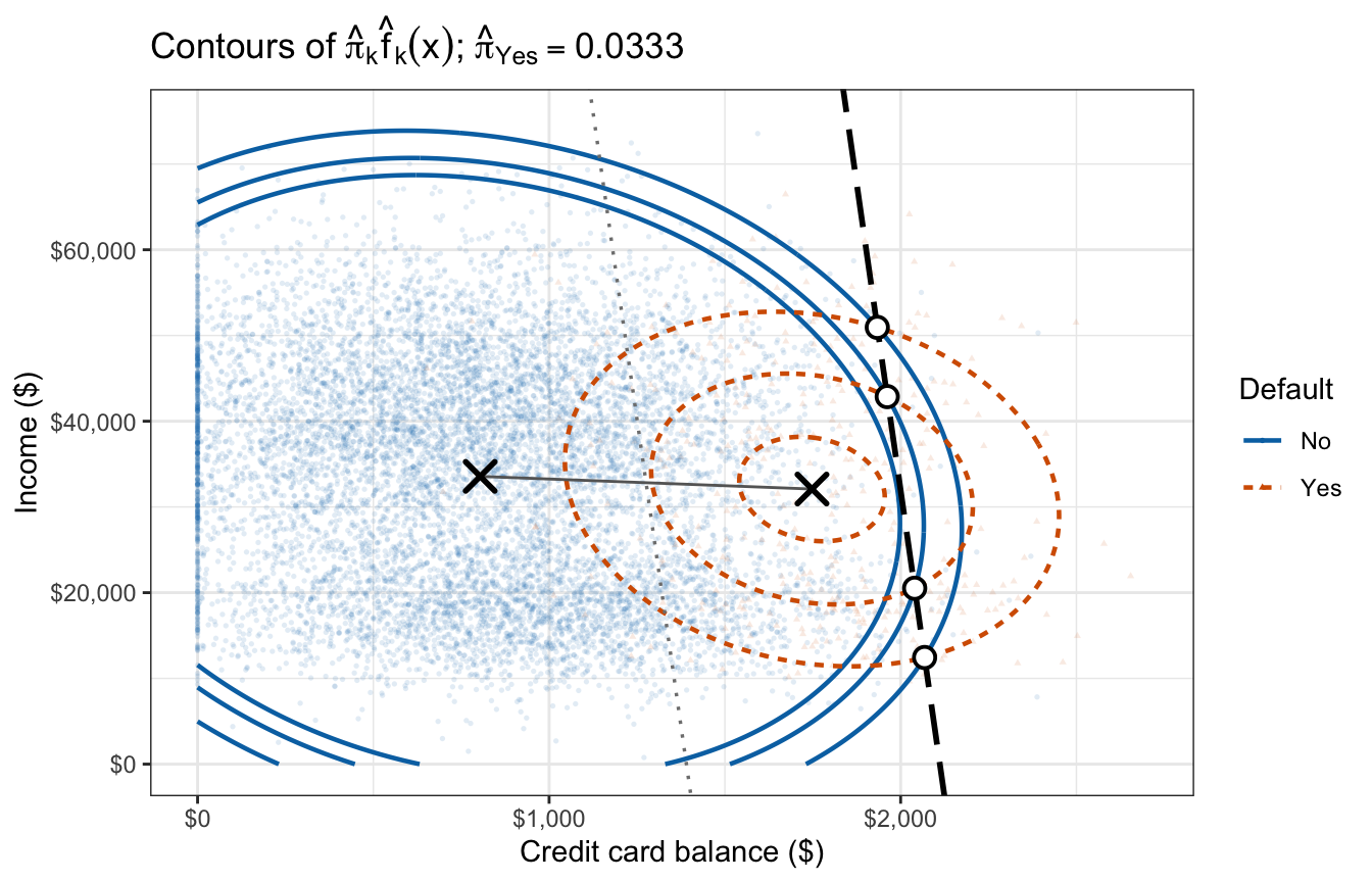
The two sets of ellipses in the first tab have the same shape and tilt, because $\hat\Sigma$ is shared, and they tilt only slightly, as the weak negative correlation implies. With equal priors the boundary passes through the midpoint of the grey segment, as the algebra requires, and through every circled crossing. With the estimated priors the defaulter surface is scaled by $\hat\pi_{\text{Yes}} = 0.0333$, so its contours shrink to small ellipses around the defaulters’ mean, and the boundary, still through the circled crossings, moves parallel to the equal-prior line toward the defaulters, because the prior enters only $\beta_0$.

The estimated boundary is nearly vertical: across the whole observed range of income, LDA’s balance threshold shifts by only $254, against a range of balance of $2,654.

13.3.5 Multiple logistic regression comparison

The log posterior odds $\hat\beta_0 + x^\top\hat\beta$ can again be set beside a logistic regression with the same two features.

Code

additive_glm <- glm(default ~ balance + income, data = Default,
                    family = "binomial")
b_glm_2 <- coef(additive_glm)
z_income_glm <- summary(additive_glm)$coefficients["income", "z value"]

# Income difference between the classes that their balance difference
# predicts through the pooled within-class regression of income on balance.
mean_diff <- hand_2$mu["Yes", ] - hand_2$mu["No", ]
income_diff_predicted <- hand_2$Sigma[1, 2] / hand_2$Sigma[1, 1] * mean_diff[1]

# Income coefficients are reported per $1,000 of income.
coef_table_2 <- tibble(
  term = c("Intercept $\\hat\\beta_0$", "`balance` $\\hat\\beta_1$",
           "`income` $\\hat\\beta_2$, per \\$1,000"),
  lda = c(hand_2$beta0, hand_2$beta[1], 1000 * hand_2$beta[2]),
  glm = c(b_glm_2[1], b_glm_2[2], 1000 * b_glm_2[3])
) |>
  mutate(across(c(lda, glm), \(v) sprintf("%.6f", v))) |>
  knitr::kable(col.names = c("Coefficient", "LDA", "Logistic regression"),
               align = "lcc")

income_levels <- quantile(Default$income, c(0.25, 0.5, 0.75))
income_level_names <- c("lower quartile", "median", "upper quartile")
x_star_lda_2 <- threshold_at(hand_2$beta0, hand_2$beta[1], hand_2$beta[2],
                             income_levels)
x_star_glm_2 <- threshold_at(b_glm_2[1], b_glm_2[2], b_glm_2[3],
                             income_levels)

boundary_lines <- tibble(
  model = c("LDA", "Logistic regression"),
  intercept = c(-hand_2$beta0 / hand_2$beta[2], -b_glm_2[1] / b_glm_2[3]),
  slope = c(-hand_2$beta[1] / hand_2$beta[2], -b_glm_2[2] / b_glm_2[3])
)

# Boundary lines take the models' colors as fixed colors, because the color
# scale already encodes default; linetype carries the legend.
boundary_layers <- function(lines) {
  list(
    geom_abline(data = filter(lines, model == "LDA"),
                aes(intercept = intercept, slope = slope, linetype = model),
                color = model_colors[["LDA"]], linewidth = 1),
    geom_abline(data = filter(lines, model == "Logistic regression"),
                aes(intercept = intercept, slope = slope, linetype = model),
                color = model_colors[["Logistic regression"]], linewidth = 1),
    scale_linetype_manual(values = c("solid", "dashed")),
    guides(linetype = guide_legend(
      override.aes = list(color = unname(model_colors))))
  )
}

boundary_plot <- scatter_base +
  boundary_layers(boundary_lines) +
  coord_cartesian(xlim = range(Default$balance),
                  ylim = range(Default$income)) +
  labs(linetype = "Boundary",
       title = "Decision boundaries in the (balance, income) plane")

# Posterior probability against balance at three fixed incomes.
income_facet <- function(v) {
  factor(v, levels = unname(income_levels),
         labels = sprintf("Income $%s (%s)", dollars(income_levels),
                          income_level_names))
}
posterior_grid_2 <- expand_grid(balance = seq(0, 2800, length.out = 400),
                                income = unname(income_levels))
posterior_curves_2 <- posterior_grid_2 |>
  mutate(LDA = predict(additive_lda, newdata = posterior_grid_2)$posterior[, "Yes"],
         `Logistic regression` = predict(additive_glm,
                                         newdata = posterior_grid_2,
                                         type = "response"),
         income_label = income_facet(income)) |>
  pivot_longer(c(LDA, `Logistic regression`), names_to = "model",
               values_to = "p_hat")

posterior_plot_2 <- ggplot(posterior_curves_2, aes(x = balance, y = p_hat)) +
  geom_hline(yintercept = 0.5, color = "grey60") +
  geom_line(aes(color = model, linetype = model), linewidth = 0.9) +
  facet_wrap(~ income_label, nrow = 1) +
  scale_color_manual(values = model_colors) +
  scale_y_continuous(breaks = c(0, 0.5, 1)) +
  scale_x_continuous(labels = dollar_labels) +
  labs(x = "Credit card balance ($)", y = "P(default = Yes)",
       color = "Model", linetype = "Model",
       title = "Posterior probability of default at three incomes")

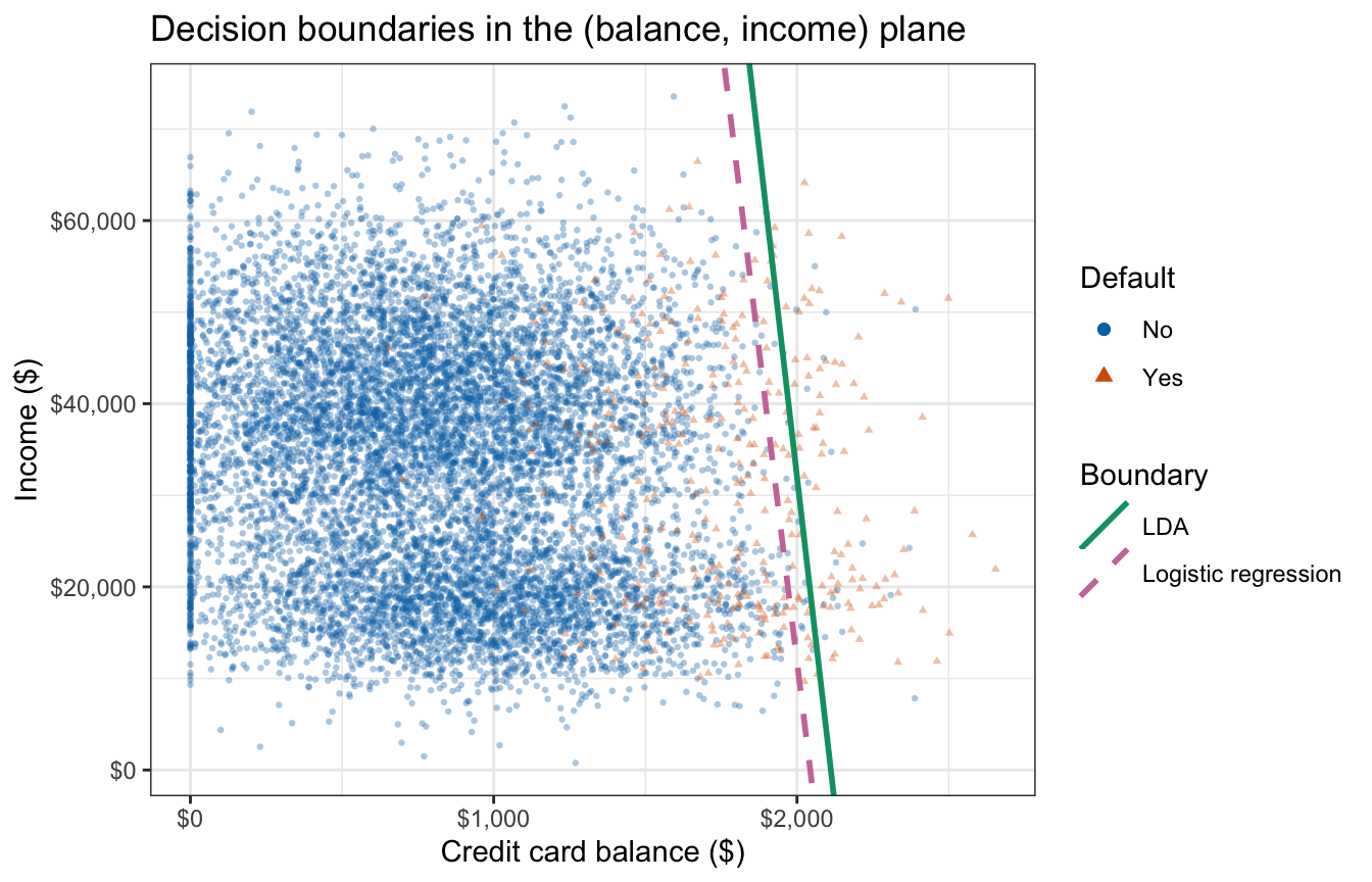
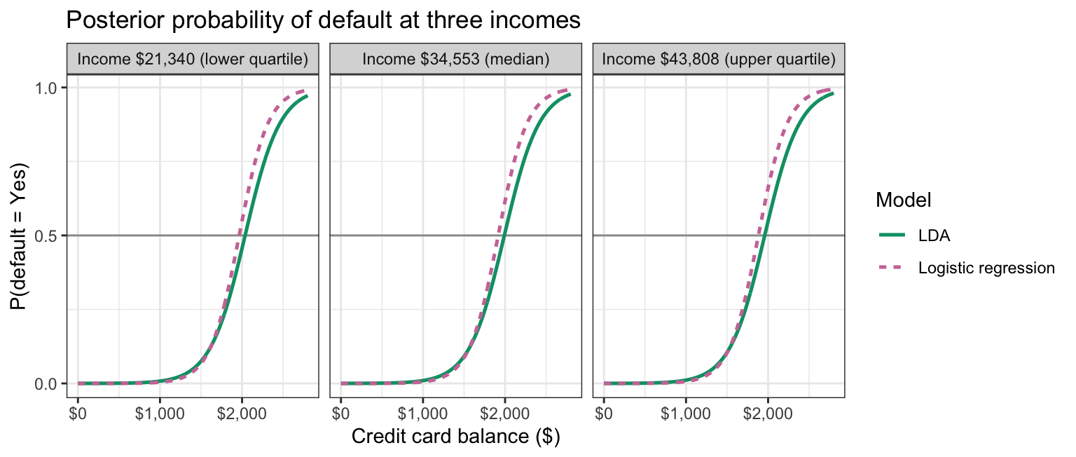
The table gives LDA’s $\hat\beta_0$ and $\hat\beta$ beside the coefficients of the logistic regression with the same two features. The first tab below draws each model’s decision boundary over the scatterplot of income against balance, LDA’s as a solid green line and logistic regression’s as a dashed pink one. The second plots each model’s posterior probability of default against balance at the lower quartile, median, and upper quartile of income, with a grey line at $0.5$.

Coefficient	LDA	Logistic regression
Intercept $\hat\beta_0$	-9.864558	-11.540468
`balance` $\hat\beta_1$	0.004672	0.005647
`income` $\hat\beta_2$, per $1,000	0.016320	0.020809

The intercept $\hat\beta_0 = -9.865$ is the log posterior odds of default for a customer with no balance and no income, an extrapolation, since the lowest recorded income is $772. The balance slope plays the same role as before. The income slope, $0.0163$ per $1,000, is positive: at a fixed balance, LDA assigns a slightly higher posterior probability of default to a customer with a higher income, although defaulters’ mean income is the lower of the two. Multiplying by $\hat\Sigma^{-1}$ adjusts each feature for the other. With the pooled within-class correlation of $-0.155$, defaulters’ higher balances predict a mean income $4,309 below non-defaulters’, but it is only $1,477 below; the positive slope reflects that excess. Logistic regression’s income coefficient, $0.0208$ per $1,000, is also positive, with $z = 4.17$; it too compares customers with the same balance. Applying the logistic function to $\hat\beta_0 + x^\top\hat\beta$ again reproduces predict()’s posterior probabilities, to within $1 \times 10^{-14}$.

Per overall standard deviation, balance moves LDA’s log posterior odds by 2.26 and income by only 0.22. The coefficients of the linear discriminant printed by MASS::lda() are proportional to the LDA column of the table: dividing each printed coefficient by the corresponding entry of $\hat\beta = \hat\Sigma^{-1}\left(\hat\mu_{\text{Yes}} - \hat\mu_{\text{No}}\right)$ gives 0.4775 for both.

Read as a balance threshold, LDA’s boundary sits at $2,037 for a customer at the lower quartile of income and $1,959 at the upper quartile; logistic regression’s sits at $1,965 and $1,882. In both models the threshold falls as income rises, and logistic regression’s lies to the left of LDA’s. At each income the LDA posterior curve is flatter than the logistic regression curve and crosses $0.5$ further right.

13.4 Conclusion

A generative classifier models the distribution of the features within each class, $f_k(x)$, and the prior probability of each class, $\pi_k$, and combines them through Bayes’ theorem into the posterior probability $p_k(x) = \pi_k f_k(x) / \sum_l \pi_l f_l(x)$. Assigning each observation to the class with the largest posterior probability is the Bayes classifier, which minimizes the expected error rate; a generative classifier approximates it by estimating $\pi_k$ and $f_k$ from training data.

Linear discriminant analysis assumes Gaussian class-conditional densities with class-specific means and a covariance matrix shared by every class. Because the covariance is shared, the quadratic term in $x$ is the same for every class, so it can be dropped from the discriminant functions $\delta_k(x)$, leaving them linear in $x$ and a decision boundary that is a point, a line, or a hyperplane. With two classes the log posterior odds are linear in the features, the same form as logistic regression, but the coefficients come from closed-form estimates from the joint likelihood of features and responses rather than from the iteratively maximized conditional likelihood of logistic regression. The class proportions and class means maximize that joint likelihood, and the pooled variance or covariance matrix is its maximizer rescaled to be unbiased. A smaller prior probability moves the boundary toward that class’s mean, and past it when the prior is small enough.

The next lecture evaluates classifiers, using this lecture’s LDA and logistic regression fits: the confusion matrix, sensitivity and specificity, the choice of classification threshold, and the ROC curve and AUC. The lecture after it relaxes LDA’s shared covariance assumption with quadratic discriminant analysis and naive Bayes.