14 Classifier Evaluation

Learning objectives

After this lecture you should be able to

construct a confusion matrix at a stated threshold (or a $K \times K$ confusion matrix for $K$ classes), compute the error rate, sensitivity, and specificity from it, and explain how sensitivity and specificity trade off as the threshold moves,
interpret an ROC curve and its AUC, the area under the curve, for which larger values (at most 1) generally indicate a better classifier, compute the AUC from the points of an ROC curve by the trapezoid rule, and explain why the ROC curve and the AUC depend on a classifier only through how it orders the observations, and
compare classifiers fit to the same observations, including models fit separately within the strata of a categorical variable, by error rate, sensitivity, specificity, and AUC, and explain why training rates overstate performance on new observations.

14.1 Credit card classifiers

14.1.1 Credit card default data

Question. How well do the LDA and logistic regression classifiers of the Linear Discriminant Analysis lecture identify the credit card customers who will default, and which kinds of mistakes do they make?

Data. ISLR2::Default is a simulated data set of 10,000 credit card customers. The response is default, with Yes the positive class. The features are balance, the customer’s monthly credit card balance in dollars, and income, the customer’s income in dollars; student (Yes/No) splits the customers in the Student strata section.

The table gives each default class’s number and proportion of customers and the mean, standard deviation, and number of zero values of its balances. The figure plots income against balance for every customer, with defaulters and non-defaulters distinguished by color and shape.

Code

dollars <- function(v) format(round(v), big.mark = ",")
# Axis labels such as $60,000, without the scales package.
dollar_labels <- function(v) {
  ifelse(is.na(v), NA,
         paste0("$", format(v, big.mark = ",", scientific = FALSE, trim = TRUE)))
}

class_summary <- Default |>
  group_by(default) |>
  summarize(n = n(), prop = n() / nrow(Default),
            mean_balance = mean(balance), sd_balance = sd(balance),
            n_zero = sum(balance == 0), .groups = "drop")
summary_of <- function(k, col) class_summary[[col]][class_summary$default == k]

class_summary_table <- class_summary |>
  transmute(default, n = format(n, big.mark = ","),
            prop = sprintf("%.4f", prop),
            mean_balance = dollars(mean_balance),
            sd_balance = dollars(sd_balance),
            n_zero = format(n_zero, big.mark = ",")) |>
  knitr::kable(col.names = c("Default", "Customers", "Proportion",
                             "Mean balance (\\$)", "SD of balance (\\$)",
                             "Zero balances"),
               align = "cccccc")

# Defaulters are drawn last so they are not hidden under non-defaulters.
scatter_base <- ggplot(arrange(Default, default),
                       aes(x = balance, y = income)) +
  geom_point(aes(color = default, shape = default), alpha = 0.35,
             size = 0.8) +
  scale_color_manual(values = class_colors) +
  scale_shape_manual(values = c(16, 17)) +
  guides(color = guide_legend(override.aes = list(alpha = 1, size = 2))) +
  scale_x_continuous(labels = dollar_labels) +
  scale_y_continuous(labels = dollar_labels) +
  labs(x = "Credit card balance ($)", y = "Income ($)", color = "Default",
       shape = "Default")

eda_scatter <- scatter_base +
  labs(title = "ISLR2::Default, income against balance")

Default	Customers	Proportion	Mean balance ($)	SD of balance ($)	Zero balances
No	9,667	0.9667	804	456	499
Yes	333	0.0333	1,748	341	0

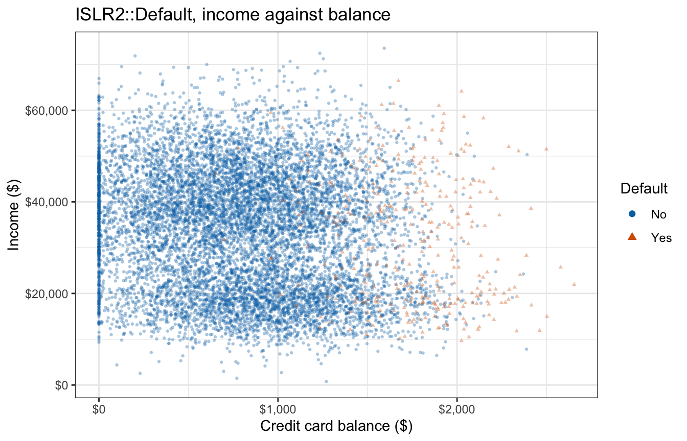
Only 333 customers, a proportion of 0.0333, defaulted. Defaulters sit at larger balances, across nearly the whole range of income, and the two classes’ clouds overlap heavily.

14.1.2 Fitted classifiers

The LDA lecture fit four classifiers to all of these customers: LDA and logistic regression with balance alone, and LDA and logistic regression with balance and income. Each gives every customer a posterior probability of default, $\hat p(x)$, and this lecture evaluates those probabilities as scores. The figure draws the two-feature classifiers’ decision boundaries, where $\hat p(x) = 0.5$, over the scatterplot, LDA’s as a solid green line and logistic regression’s as a dashed pink one.

Code

# Estimates of pi_k, mu_k, Sigma and the implied log posterior odds
# beta0 + x' beta of the second class, as in the LDA lecture.
lda_by_hand <- function(X, y) {
  X <- as.matrix(X)
  classes <- levels(y)
  n <- nrow(X)
  K <- length(classes)
  pi_hat <- as.numeric(table(y)) / n
  mu_hat <- do.call(rbind, lapply(classes, function(k) {
    colMeans(X[y == k, , drop = FALSE])
  }))
  rownames(mu_hat) <- classes
  Sigma_hat <- Reduce(`+`, lapply(classes, function(k) {
    Z <- sweep(X[y == k, , drop = FALSE], 2, mu_hat[k, ])
    crossprod(Z)
  })) / (n - K)
  beta  <- solve(Sigma_hat, mu_hat[2, ] - mu_hat[1, ])
  beta0 <- log(pi_hat[2] / pi_hat[1]) -
    0.5 * (sum(mu_hat[2, ] * solve(Sigma_hat, mu_hat[2, ])) -
           sum(mu_hat[1, ] * solve(Sigma_hat, mu_hat[1, ])))
  list(pi = pi_hat, mu = mu_hat, Sigma = Sigma_hat,
       beta0 = beta0, beta = beta)
}

# Balance alone.
hand_1 <- lda_by_hand(Default["balance"], Default$default)
balance_lda <- MASS::lda(default ~ balance, data = Default)
balance_glm <- glm(default ~ balance, data = Default, family = "binomial")
post_1 <- predict(balance_lda)$posterior[, "Yes"]

# Balance and income.
additive_lda <- MASS::lda(default ~ balance + income, data = Default)
hand_2 <- lda_by_hand(Default[c("balance", "income")], Default$default)
post_lda_2 <- predict(additive_lda)$posterior[, "Yes"]
additive_glm <- glm(default ~ balance + income, data = Default,
                    family = "binomial")
b_glm_2 <- coef(additive_glm)
z_income_glm <- summary(additive_glm)$coefficients["income", "z value"]
post_glm_2 <- fitted(additive_glm)

income_levels <- quantile(Default$income, c(0.25, 0.5, 0.75))
# A boundary read as a balance threshold at a given income.
threshold_at <- function(b0, b1, b2, inc) -(b0 + b2 * inc) / b1

boundary_lines <- tibble(
  model = c("LDA", "Logistic regression"),
  intercept = c(-hand_2$beta0 / hand_2$beta[2], -b_glm_2[1] / b_glm_2[3]),
  slope = c(-hand_2$beta[1] / hand_2$beta[2], -b_glm_2[2] / b_glm_2[3])
)

# Boundary lines take the models' colors as fixed colors, because the color
# scale already encodes default; linetype carries the legend.
boundary_layers <- function(lines) {
  list(
    geom_abline(data = filter(lines, model == "LDA"),
                aes(intercept = intercept, slope = slope, linetype = model),
                color = model_colors[["LDA"]], linewidth = 1),
    geom_abline(data = filter(lines, model == "Logistic regression"),
                aes(intercept = intercept, slope = slope, linetype = model),
                color = model_colors[["Logistic regression"]], linewidth = 1),
    scale_linetype_manual(values = c("solid", "dashed")),
    guides(linetype = guide_legend(
      override.aes = list(color = unname(model_colors))))
  )
}

boundary_plot <- scatter_base +
  boundary_layers(boundary_lines) +
  coord_cartesian(xlim = range(Default$balance),
                  ylim = range(Default$income)) +
  labs(linetype = "Boundary",
       title = "Decision boundaries in the (balance, income) plane")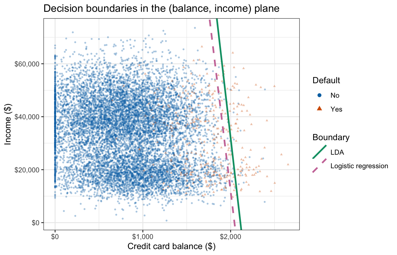

The two boundaries are nearly vertical and close together, with logistic regression’s slightly to the left of LDA’s. Customers to the right of a boundary are classified as defaulters, and many defaulters lie to its left.

14.2 Classifier evaluation

An error rate counts every mistake the same way. Failing to flag a customer who goes on to default and flagging a customer who does not are different mistakes with different costs, and a classifier can have a small error rate while making almost every mistake of one kind. The classification lecture introduced the confusion matrix, which separates the mistakes; this section develops it in full for two classes and for $K$ classes, and adds the ROC curve and AUC, which summarize a two-class classifier at every threshold. The running example is the LDA classifier with balance and income.

The figure shows, for each true default class, the histogram of the balance and income LDA classifier’s log posterior odds of default, on the density scale, with a dotted line at $0$, where the classifier’s estimated probability of default, $\hat p(x)$, equals $0.5$.

Code

# Log posterior odds of default from the balance + income LDA, binned once so
# this figure and the threshold slider below share the same bars.
lda_score <- qlogis(post_lda_2)
score_breaks <- seq(floor(min(lda_score)), ceiling(max(lda_score)), by = 0.5)
class_label <- c(No = "No (negative)", Yes = "Yes (positive)")
slider_bins <- map(c("No", "Yes"), \(k) {
  h <- hist(lda_score[Default$default == k], breaks = score_breaks,
            plot = FALSE)
  tibble(class = class_label[[k]], x0 = head(h$breaks, -1),
         x1 = tail(h$breaks, -1), density = h$density)
}) |>
  list_rbind()

score_by_class <- tibble(score = lda_score, default = Default$default) |>
  group_by(default) |>
  summarize(median = median(score), below_0 = mean(score <= 0),
            above_0 = mean(score > 0), .groups = "drop")
score_of <- function(k, col) score_by_class[[col]][score_by_class$default == k]

score_hist_plot <- tibble(score = lda_score, default = Default$default) |>
  ggplot(aes(x = score)) +
  geom_histogram(aes(y = after_stat(density)), breaks = score_breaks,
                 fill = "grey80", color = "grey55") +
  geom_vline(xintercept = 0, linetype = "dotted") +
  facet_wrap(~ default, ncol = 1, labeller = label_both) +
  labs(x = "LDA log posterior odds of default", y = "Density",
       title = "LDA (balance + income) scores within each true class")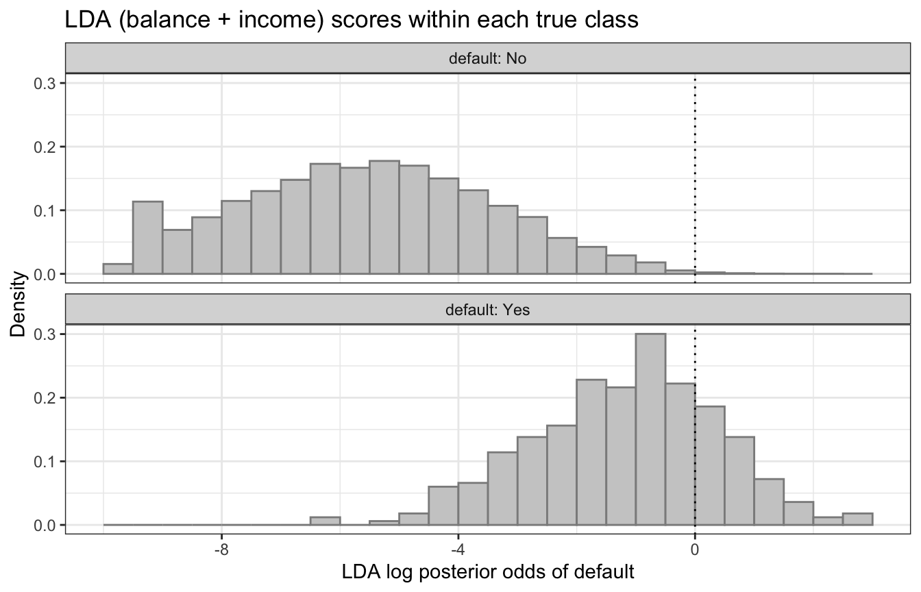

The defaulters’ scores sit well to the right of the non-defaulters’ (medians -1.06 and -5.56), but the two histograms overlap: 76.9% of defaulters score at or below $0$, and 0.2% of non-defaulters above it. Any threshold inside the overlap makes two kinds of mistake, defaulters to its left and non-defaulters to its right.

14.2.1 Confusion matrix

With two classes, call the class of interest positive and the other negative. For a classifier that produces an estimated probability $\hat p(x)$ of the positive class, a threshold $t$ turns probabilities into classes: predict positive when $\hat p(x) > t$.

As in the classification lecture, a confusion matrix cross-tabulates the true class against the predicted class:

Code

confusion_template <- tibble(
  Truth = c("Positive", "Negative"),
  `Predicted positive` = c("True positive (TP)", "False positive (FP)"),
  `Predicted negative` = c("False negative (FN)", "True negative (TN)")
) |>
  knitr::kable(align = "lcc")

Truth	Predicted positive	Predicted negative
Positive	True positive (TP)	False negative (FN)
Negative	False positive (FP)	True negative (TN)

where

$TP$ is the number of positive observations predicted positive,
$FN$ is the number of positive observations predicted negative,
$FP$ is the number of negative observations predicted positive, and
$TN$ is the number of negative observations predicted negative.

In the score histograms above, with $t = 0.5$, $TP$ and $FN$ count the defaulters to the right and left of the dotted line, and $FP$ and $TN$ the non-defaulters to its right and left. The diagonal holds the correct classifications, so the error rate is $(FP + FN)/n$.

Classifying each credit card customer as a defaulter when $\hat p(x) > 0.5$, the LDA classifier with balance and income produces this confusion matrix:

Code

confusion_counts <- function(p_hat, t) {
  truth <- Default$default == "Yes"
  pred  <- p_hat > t
  c(TP = sum(truth & pred), FN = sum(truth & !pred),
    FP = sum(!truth & pred), TN = sum(!truth & !pred))
}

cm_lda_05 <- confusion_counts(post_lda_2, 0.5)
# A lower threshold, compared with 0.5 below.
t_low <- 0.2

confusion_lda_table <- tibble(
  Truth = c("Yes", "No"),
  `Predicted Yes` = c(cm_lda_05["TP"], cm_lda_05["FP"]),
  `Predicted No`  = c(cm_lda_05["FN"], cm_lda_05["TN"])
) |>
  mutate(Total = `Predicted Yes` + `Predicted No`) |>
  mutate(across(-Truth, \(v) format(v, big.mark = ","))) |>
  knitr::kable(align = "lccc")

metrics <- function(cm) {
  c(error = unname((cm["FP"] + cm["FN"]) / sum(cm)),
    sensitivity = unname(cm["TP"] / (cm["TP"] + cm["FN"])),
    specificity = unname(cm["TN"] / (cm["TN"] + cm["FP"])))
}
m_lda_05 <- metrics(cm_lda_05)

Truth	Predicted Yes	Predicted No	Total
Yes	77	256	333
No	20	9,647	9,667

The classifier misclassifies 276 of 10,000 customers, an error rate of 2.76%, against the 3.33% of the classifier that predicts No for everyone. The error rate is small because the 9,667 non-defaulters, nearly all classified correctly, dominate it, even though 256 of the 276 errors are missed defaulters.

These are training error rates: the customers being classified are the ones the model was fit to, so they are optimistic estimates of performance on new customers, as the classification lecture discussed. Estimating test error from the training data alone is the subject of the resampling unit.

14.2.2 Sensitivity and specificity

Dividing each row by its total gives two rates that condition on the true class:

\[\text{Sensitivity} = \frac{TP}{TP + FN}, \qquad \text{Specificity} = \frac{TN}{TN + FP},\]

where

sensitivity, also called recall or the true positive rate (TPR), is the proportion of positive observations the classifier catches, an estimate of $P\left(\hat y(X) = \text{positive} \mid Y = \text{positive}\right)$, and
specificity, also called the true negative rate, is the proportion of negative observations the classifier correctly leaves alone, an estimate of $P\left(\hat y(X) = \text{negative} \mid Y = \text{negative}\right)$.

Their complements are error rates within each true class: $1 - \text{sensitivity} = FN/(TP + FN)$ is the false negative rate, and $1 - \text{specificity} = FP/(TN + FP)$ is the false positive rate (FPR).

In the credit card confusion matrix, of the 333 customers who defaulted the classifier flags only 77, a sensitivity of 23.1%. Of the 9,667 who did not, it correctly leaves alone 9,647, a specificity of 99.8%.

14.2.3 Multiple classes

With $K$ classes the confusion matrix is $K \times K$, with true classes in the rows and predicted classes in the columns:

Code

k_labels <- c("1", "2", "$\\vdots$", "$K$")
cell <- function(k, j) {
  ifelse(k == "$\\vdots$" | j == "$\\vdots$", "$\\vdots$",
         sprintf("$n_{%s%s}$", gsub("\\$", "", k), gsub("\\$", "", j)))
}
confusion_template_k <- tibble(Truth = k_labels) |>
  mutate(`Predicted 1` = cell(Truth, "1"),
         `Predicted 2` = cell(Truth, "2"),
         `$\\cdots$`   = ifelse(Truth == "$\\vdots$", "$\\ddots$", "$\\cdots$"),
         `Predicted $K$` = cell(Truth, "$K$")) |>
  knitr::kable(align = "lcccc", escape = FALSE)

Truth	Predicted 1	Predicted 2	$\cdots$	Predicted $K$
1	$n_{11}$	$n_{12}$	$\cdots$	$n_{1K}$
2	$n_{21}$	$n_{22}$	$\cdots$	$n_{2K}$
$\vdots$	$\vdots$	$\vdots$	$\ddots$	$\vdots$
$K$	$n_{K1}$	$n_{K2}$	$\cdots$	$n_{KK}$

where

$n_{kj}$ is the number of observations in true class $k$ predicted to be in class $j$, so the diagonal entries $n_{kk}$ are the correct classifications.

The error rate is $1 - \sum_{k=1}^K n_{kk} / n$. Sensitivity and specificity are defined one class at a time, one versus the rest: treat class $k$ as positive and the other $K - 1$ classes together as negative, which collapses the table to two-by-two. Class $k$’s rates are

\[\text{Sensitivity}_k = \frac{n_{kk}}{\sum_{j=1}^K n_{kj}}, \qquad \text{Specificity}_k = \frac{\sum_{l \ne k} \sum_{j \ne k} n_{lj}}{\sum_{l \ne k} \sum_{j=1}^K n_{lj}},\]

where

the sensitivity’s denominator is the number of observations in class $k$, and its numerator the number of those predicted to be in class $k$, and
the specificity’s denominator is the number of observations in the other classes, and its numerator the number of those predicted to be in some class other than $k$, whether or not it is their own.

With $K$ classes the threshold $t = 0.5$ generalizes to assigning each observation to the class with the largest estimated posterior probability; with $K = 2$ the two rules coincide. Other thresholds, and the ROC curve and AUC built from them, are two-class tools, and the rest of this section returns to two classes.

Beyond this course

ROC curves and AUC extend to $K > 2$ classes by averaging the AUCs of the $K$ one-versus-rest problems, or of all $K(K-1)/2$ pairs of classes. Logistic regression as developed in this course is also a two-class method; its multi-class extension, multinomial logistic regression, is not covered in this course.

14.2.4 Classification threshold

The threshold $t = 0.5$ is the Bayes classifier’s: if $\hat p(x)$ equalled the true $p_2(x)$, the posterior probability of the positive class, it would minimize the expected error rate. An estimated $\hat p(x)$ carries no such guarantee, and even for the Bayes classifier the overall error rate need not be the quantity of interest.

Lowering $t$ enlarges the set $\left\{x : \hat p(x) > t\right\}$ of feature values classified positive, so every observation predicted positive at the old threshold is still predicted positive at the new one. Consequently $TP$ and $FP$ can only grow while $FN$ and $TN$ can only shrink: sensitivity rises or stays the same, and specificity falls or stays the same. Raising $t$ does the reverse, so no threshold improves both.

Beyond this course

If the two mistakes have known costs, $c_{FN}$ for a missed positive and $c_{FP}$ for a false alarm, the expected cost of predicting positive at $x$ is $c_{FP}\left[1 - p_2(x)\right]$ and of predicting negative is $c_{FN}\, p_2(x)$. Predicting positive is the cheaper choice exactly when $p_2(x) > c_{FP}/(c_{FP} + c_{FN})$, so that ratio is the cost-minimizing threshold. Equal costs recover $t = 0.5$.

A credit card company that wants to catch more of its eventual defaulters can lower the threshold. The figure below tracks four rates of the LDA classifier with balance and income as $t$ moves from $0$ to $0.5$ — the overall error rate, sensitivity (the true positive rate), specificity (the true negative rate), and the false positive rate ($1 - \text{specificity}$) — with dotted lines at $t = 0.2$ and $t = 0.5$. The checkboxes choose which rates are drawn; the false positive rate starts unchecked because it mirrors specificity. The table below the figure gives the confusion-matrix counts and rates at $t = 0.5$ and $t = 0.2$ for LDA with balance alone, LDA with balance and income, and the logistic regression with balance and income.

Code

threshold_rates <- tibble(t = seq(0, 0.5, by = 0.005)) |>
  mutate(m = map(t, \(tt) metrics(confusion_counts(post_lda_2, tt))),
         `Overall error rate` = map_dbl(m, "error"),
         `Sensitivity (true positive rate)` = map_dbl(m, "sensitivity"),
         `Specificity (true negative rate)` = map_dbl(m, "specificity"),
         `False positive rate (1 - specificity)` =
           map_dbl(m, \(v) 1 - v[["specificity"]])) |>
  select(-m) |>
  pivot_longer(-t, names_to = "rate", values_to = "value")

# Training error rate at every distinct posterior probability used as t;
# the error rate only changes when t passes an observation's score.
min_error_threshold <- function(p_hat) {
  cand <- sort(unique(p_hat))
  err  <- map_dbl(cand, \(tt) metrics(confusion_counts(p_hat, tt))[["error"]])
  c(t = cand[which.min(err)], error = min(err))
}
min_err_lda <- min_error_threshold(post_lda_2)
min_err_glm <- min_error_threshold(post_glm_2)

cm_lda1_05  <- confusion_counts(post_1, 0.5)
cm_lda1_low <- confusion_counts(post_1, t_low)
cm_lda_low  <- confusion_counts(post_lda_2, t_low)
cm_glm_05   <- confusion_counts(post_glm_2, 0.5)
cm_glm_low  <- confusion_counts(post_glm_2, t_low)
m_lda1_05   <- metrics(cm_lda1_05)
m_lda1_low  <- metrics(cm_lda1_low)
m_lda_low   <- metrics(cm_lda_low)
m_glm_05    <- metrics(cm_glm_05)
m_glm_low   <- metrics(cm_glm_low)

compare_table <- tibble(
  Model = rep(c("LDA, balance", "LDA, balance + income",
                "Logistic regression, balance + income"), each = 2),
  t = rep(c(0.5, t_low), 3),
  cm = list(cm_lda1_05, cm_lda1_low, cm_lda_05, cm_lda_low,
            cm_glm_05, cm_glm_low)
) |>
  mutate(TP = map_dbl(cm, "TP"), FN = map_dbl(cm, "FN"),
         FP = map_dbl(cm, "FP"), TN = map_dbl(cm, "TN"),
         m = map(cm, metrics),
         error = map_dbl(m, "error"),
         sensitivity = map_dbl(m, "sensitivity"),
         specificity = map_dbl(m, "specificity")) |>
  select(-cm, -m) |>
  mutate(across(c(TP, FN, FP, TN), \(v) format(v, big.mark = ",")),
         across(c(error, sensitivity, specificity),
                \(v) sprintf("%.4f", v))) |>
  knitr::kable(col.names = c("Model", "Threshold", "TP", "FN", "FP", "TN",
                             "Error rate", "Sensitivity", "Specificity"),
               align = "lcccccccc")

rateNames = ["Overall error rate", "Sensitivity (true positive rate)",
             "Specificity (true negative rate)",
             "False positive rate (1 - specificity)"]
rateStyles = ({
  "Overall error rate": {stroke: "black", dash: "none"},
  "Sensitivity (true positive rate)": {stroke: "#D55E00", dash: "8,4"},
  "Specificity (true negative rate)": {stroke: "#0072B2", dash: "2,4"},
  "False positive rate (1 - specificity)": {stroke: "#009E73", dash: "12,4,2,4"}
})
viewof shownRates = Inputs.checkbox(rateNames, {
  value: rateNames.slice(0, 3),
  format: name => html`<span style="display: inline-flex; align-items: center; gap: 0.4em">
    <svg width="36" height="10"><line x1="2" y1="5" x2="34" y2="5"
      stroke="${rateStyles[name].stroke}" stroke-width="2.5"
      stroke-dasharray="${rateStyles[name].dash}" stroke-linecap="round"/></svg>${name}</span>`
})

{
  const rates = transpose(threshold_rates);
  return Plot.plot({
    width: 640, height: 340,
    marginTop: 24,
    x: {domain: [0, 0.5], label: "Threshold t"},
    y: {domain: [0, 1], label: "Rate", grid: true},
    marks: [
      Plot.ruleX(threshold_marks, {stroke: "gray", strokeDasharray: "2,3"}),
      Plot.text(threshold_marks, {x: d => d, y: 1, text: d => `t = ${d}`,
                                  dy: -12, fill: "gray"}),
      ...rateNames.filter(r => shownRates.includes(r)).map(r =>
        Plot.line(rates.filter(d => d.rate === r),
                  {x: "t", y: "value", stroke: rateStyles[r].stroke,
                   strokeDasharray: rateStyles[r].dash, strokeWidth: 2.5,
                   strokeLinecap: "round"}))
    ]
  });
}

Model	Threshold	TP	FN	FP	TN	Error rate	Sensitivity	Specificity
LDA, balance	0.5	76	257	24	9,643	0.0281	0.2282	0.9975
LDA, balance	0.2	195	138	236	9,431	0.0374	0.5856	0.9756
LDA, balance + income	0.5	77	256	20	9,647	0.0276	0.2312	0.9979
LDA, balance + income	0.2	189	144	240	9,427	0.0384	0.5676	0.9752
Logistic regression, balance + income	0.5	108	225	38	9,629	0.0263	0.3243	0.9961
Logistic regression, balance + income	0.2	200	133	271	9,396	0.0404	0.6006	0.9720

As $t$ falls from $0.5$, sensitivity rises steadily while specificity stays near $1$, and the false positive rate near $0$, until $t$ is small. The overall error rate, dominated by the 9,667 non-defaulters, follows the false positive rate: nearly flat over most of the range, then climbing sharply as $t$ approaches $0$ and almost every customer is flagged.

The overall error rate need not be smallest at $t = 0.5$. LDA’s training error rate is lowest near $t = 0.427$, at 2.61%, against 2.76% at $t = 0.5$. The logistic regression’s is lowest near $t = 0.504$, at 2.61%, against 2.63% at $t = 0.5$.

In the table, lowering the threshold to $t = 0.2$ raises the two-feature LDA classifier’s sensitivity from 23.1% to 56.8%, at the cost of specificity falling from 99.8% to 97.5% and the overall error rate rising from 2.76% to 3.84%. Adding income changes LDA very little: with balance alone the error rate is 2.81% and the sensitivity 22.8% at $t = 0.5$, and 3.74% and 58.6% at $t = 0.2$. At both thresholds logistic regression flags more customers as defaulters than the two-feature LDA classifier does — 146 against 97 at $t = 0.5$ — and has the higher sensitivity and the lower specificity of the two.

14.2.5 ROC curve

The ROC curve (receiver operating characteristic curve) plots sensitivity against $1 - \text{specificity}$ — the true positive rate against the false positive rate — at every threshold. At $t = 1$ nothing is predicted positive, giving the point $(0, 0)$; at $t = 0$ everything is, giving $(1, 1)$; and the curve traces every tradeoff in between.

The ROC curve depends on a classifier only through how it orders the observations. Any strictly increasing transformation of the score — the log posterior odds $\hat\delta_2(x) - \hat\delta_1(x)$ or $\hat p(x)$ itself — sorts the observations identically, produces the same sequence of confusion matrices, and so traces the same curve. Predicting positive when $\hat p(x) > t$ is the same as predicting positive when the log posterior odds exceed the cutoff $c = \log\left[t/(1 - t)\right]$.

For the credit card LDA classifier, the slider below moves the threshold $t$; its left panel uses the same bins as the score histograms above. A line above the plots reports $t$, the cutoff $c$ on the log posterior odds, sensitivity, and specificity. The left panel draws the histograms of the classifier’s log posterior odds within each class, on the density scale, the defaulters’ with a dashed outline and the non-defaulters’ with a solid one, and a dotted vertical line at $c$; the shaded bars to the right of $c$ are the customers flagged, darker for defaulters (sensitivity) and lighter for non-defaulters (the false positive rate). The right panel marks where the classifier lands on its ROC curve, with a dashed diagonal for reference.

Code

is_yes <- Default$default == "Yes"

# Empirical ROC curve: every distinct score is a cutoff; classify positive
# when score >= cutoff.
roc_curve <- function(score, positive) {
  ord <- order(score, decreasing = TRUE)
  s   <- score[ord]
  pos <- positive[ord]
  keep <- c(diff(s) != 0, TRUE)
  tibble(fpr = c(0, cumsum(!pos)[keep] / sum(!positive)),
         tpr = c(0, cumsum(pos)[keep] / sum(positive)))
}

# Area under an ROC curve (sorted by fpr) by the trapezoid rule.
auc_trapezoid <- function(roc) {
  with(roc, sum(diff(fpr) * (head(tpr, -1) + tail(tpr, -1)) / 2))
}

# Everything the slider needs, indexed by t = 0.01, 0.02, ..., 0.99, is
# computed here and passed to the page, which only looks values up.
# Each histogram's outline, as a stair through the bin edges.
slider_outline <- slider_bins |>
  pivot_longer(c(x0, x1), values_to = "x") |>
  select(class, x, density)

slider_thresholds <- tibble(t = (1:99) / 100) |>
  mutate(cutoff = qlogis(t),
         m = map(t, \(tt) metrics(confusion_counts(post_lda_2, tt))),
         fpr = 1 - map_dbl(m, "specificity"),
         tpr = map_dbl(m, "sensitivity")) |>
  select(-m)

roc_lda_2 <- roc_curve(post_lda_2, is_yes)
slider_roc <- slice(roc_lda_2, unique(c(seq(1, n(), by = 10), n())))

viewof t = Inputs.range([0.01, 0.99], {value: 0.5, step: 0.01, label: "Threshold t"})

{
  const bins = transpose(slider_bins);
  const outline = transpose(slider_outline);
  const thresholds = transpose(slider_thresholds);
  const roc = transpose(slider_roc);
  const now = thresholds[Math.round(t * 100) - 1];
  const classes = ["No (negative)", "Yes (positive)"];
  const flagged = k => bins
    .filter(d => d.class === k && d.x1 > now.cutoff)
    .map(d => ({...d, x0: Math.max(d.x0, now.cutoff)}));

  const densityPlot = Plot.plot({
    width: 360, height: 300,
    x: {label: "LDA log posterior odds of default"},
    y: {label: "Density within class"},
    color: {domain: classes, range: slider_colors, legend: true},
    marks: [
      Plot.rect(flagged(classes[0]),
                {x1: "x0", x2: "x1", y1: 0, y2: "density", fill: "class",
                 fillOpacity: 0.2}),
      Plot.rect(flagged(classes[1]),
                {x1: "x0", x2: "x1", y1: 0, y2: "density", fill: "class",
                 fillOpacity: 0.45}),
      Plot.line(outline.filter(d => d.class === classes[0]),
                {x: "x", y: "density", stroke: "class", strokeWidth: 2}),
      Plot.line(outline.filter(d => d.class === classes[1]),
                {x: "x", y: "density", stroke: "class", strokeDasharray: "6,4",
                 strokeWidth: 2}),
      Plot.ruleX([now.cutoff], {strokeDasharray: "2,3"})
    ]
  });

  const rocPlot = Plot.plot({
    width: 300, height: 300,
    x: {domain: [0, 1], label: "False positive rate (1 − specificity)"},
    y: {domain: [0, 1], label: "True positive rate (sensitivity)"},
    marks: [
      Plot.line([[0, 0], [1, 1]], {stroke: "gray", strokeDasharray: "4,4"}),
      Plot.line(roc, {x: "fpr", y: "tpr", strokeWidth: 2}),
      Plot.dot([now], {x: "fpr", y: "tpr", r: 6, fill: "white", stroke: "black",
                       strokeWidth: 2})
    ]
  });

  return html`<p style="text-align: center"><b>t = ${t.toFixed(2)}</b>,
    cutoff c = ${now.cutoff.toFixed(2)}; sensitivity = ${now.tpr.toFixed(3)},
    specificity = ${(1 - now.fpr).toFixed(3)}</p>
    <div style="display: flex; flex-wrap: wrap; gap: 1rem; justify-content: center">
      ${densityPlot}${rocPlot}
    </div>`;
}

Moving the slider from $t = 0.9$ to $t = 0.1$ slides the cutoff left, so the shaded share of the defaulters’ histogram (sensitivity) and of the non-defaulters’ (false positive rate) both grow, and the point climbs along the curve toward $(1, 1)$. The dashed diagonal is the ROC curve of a classifier that ignores the features and predicts positive at random: its true and false positive rates are equal at every threshold. The LDA curve bows far toward the top-left corner, where sensitivity is high and the false positive rate is low.

The ROC curves below compare LDA and logistic regression with balance and income at every threshold. Their points at $t = 0.5$ (filled) and $t = 0.2$ (open) from the threshold table are marked, a triangle for LDA and a square for logistic regression, with a dashed diagonal for reference.

Code

roc_2 <- bind_rows(
  roc_lda_2 |> mutate(model = "LDA"),
  roc_curve(post_glm_2, is_yes) |> mutate(model = "Logistic regression")
)

threshold_labels <- c("t = 0.5", paste("t =", t_low))
roc_points <- tibble(
  model = rep(c("LDA", "Logistic regression"), each = 2),
  t = factor(rep(threshold_labels, 2), levels = threshold_labels),
  m = list(m_lda_05, m_lda_low, m_glm_05, m_glm_low)
) |>
  mutate(fpr = 1 - map_dbl(m, "specificity"),
         tpr = map_dbl(m, "sensitivity"))

roc_plot <- ggplot(roc_2, aes(x = fpr, y = tpr)) +
  geom_abline(intercept = 0, slope = 1, color = "grey60",
              linetype = "dashed") +
  geom_line(aes(color = model, linetype = model), linewidth = 0.9) +
  geom_point(data = roc_points, aes(shape = model, color = model, fill = t),
             size = 3, stroke = 1.2) +
  scale_color_manual(values = model_colors) +
  # Shape separates the models, filled versus open separates the thresholds.
  scale_shape_manual(values = c(24, 22)) +
  scale_fill_manual(values = c("black", "white")) +
  guides(fill = guide_legend(override.aes = list(shape = 21))) +
  coord_fixed() +
  labs(x = "False positive rate (1 - specificity)",
       y = "True positive rate (sensitivity)",
       color = "Model", linetype = "Model", shape = "Model",
       fill = "Threshold", title = "ROC curves, balance + income")

# Balance at which the two models' posterior curves cross, at the lower
# quartile, median, and upper quartile of income, and the posterior
# probability there.
posterior_both <- function(b, inc) {
  nd <- tibble(balance = b, income = inc)
  c(lda = predict(additive_lda, newdata = nd)$posterior[, "Yes"],
    glm = unname(predict(additive_glm, newdata = nd, type = "response")))
}
crossover <- tibble(income = unname(income_levels)) |>
  mutate(balance = map_dbl(income, \(i) {
           uniroot(\(b) diff(posterior_both(b, i)), c(800, 2500))$root
         }),
         p = map2_dbl(balance, income, \(b, i) posterior_both(b, i)[["lda"]]))

# Is one model's flagged set contained in the other's at a threshold?
flags_within <- function(p_inner, p_outer, t) !any(p_inner > t & p_outer <= t)
t_below <- 0.1
lda_within_glm <- flags_within(post_lda_2, post_glm_2, 0.5) &&
  flags_within(post_lda_2, post_glm_2, t_low)
glm_within_lda_below <- flags_within(post_glm_2, post_lda_2, t_below)
n_flag_lda_below <- sum(post_lda_2 > t_below)
n_flag_glm_below <- sum(post_glm_2 > t_below)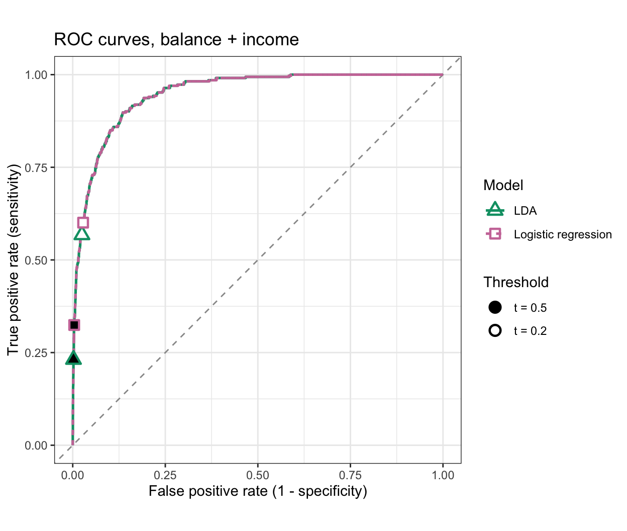

The two ROC curves lie almost on top of one another and rise steeply near the origin, well above the diagonal. Lowering $t$ from $0.5$ to 0.2 moves each model’s marked point up and slightly right along its curve. At each of these two thresholds, logistic regression’s point sits further along its nearly shared curve than LDA’s.

At the lower quartile, median, and upper quartile of income, the two models’ posterior curves cross at balances of $1,620, $1,559, and $1,516, where both give posterior probabilities of 0.125, 0.117, and 0.113. Above those balances LDA’s flatter curve lies below logistic regression’s, so a threshold above the crossing probabilities is reached by LDA only at a higher balance. At both marked thresholds, every customer LDA flags is also flagged by logistic regression. At a low threshold the order reverses: at $t = 0.1$, LDA flags 817 customers and logistic regression 805, and every customer logistic regression flags is also flagged by LDA.

14.2.6 AUC

The AUC is the area under the ROC curve, a single number summarizing the curve over all thresholds at once. The AUC is at most 1 and, generally, a larger AUC is better; the caveat below is that a classifier with the larger AUC can still be the worse one over the false positive rates that matter for an application. A classifier that ignores the features has an ROC curve along the diagonal and an AUC of 0.5; a classifier whose curve reaches the top-left corner, with sensitivity 1 at a false positive rate of 0, has an AUC of 1.

The ROC curve of a sample is a set of points $\left(\text{FPR}_m, \text{TPR}_m\right)$, one for each threshold at which the confusion matrix changes. Joining consecutive points by straight lines and adding up the trapezoids beneath them gives the AUC,

\[\text{AUC} = \sum_{m=1}^{M}\left(\text{FPR}_m - \text{FPR}_{m-1}\right)\frac{\text{TPR}_m + \text{TPR}_{m-1}}{2},\]

where

$\left(\text{FPR}_m, \text{TPR}_m\right)$ is the false and true positive rate at the $m$th point, ordered by increasing false positive rate, and
$m = 0$ is the point $(0, 0)$ and $m = M$ is the point $(1, 1)$.

For the credit card customers, the table below gives the AUC of LDA and logistic regression with balance alone and with balance and income, computed this way. In the figure, the left panel shades the area under the running example’s ROC curve, labeled with that area, with a dashed diagonal for reference. The right panel draws the ROC curves of four classifiers fit to the same customers — LDA with balance only, with income only, and with both, and a classifier that ignores the features — each labeled with its AUC.

Code

scores <- list(
  "LDA, balance" = post_1,
  "Logistic regression, balance" = fitted(balance_glm),
  "LDA, balance + income" = post_lda_2,
  "Logistic regression, balance + income" = post_glm_2
)
auc_values <- tibble(model = names(scores)) |>
  mutate(auc = map_dbl(scores, \(s) auc_trapezoid(roc_curve(s, is_yes))))
auc_of <- function(m) auc_values$auc[auc_values$model == m]
auc_table <- auc_values |>
  mutate(auc = sprintf("%.5f", auc)) |>
  knitr::kable(col.names = c("Model", "AUC"), align = "lc")

auc_area_plot <- ggplot(roc_lda_2, aes(x = fpr, y = tpr)) +
  geom_ribbon(aes(ymin = 0, ymax = tpr), fill = "grey70", alpha = 0.6) +
  geom_abline(intercept = 0, slope = 1, color = "grey40",
              linetype = "dashed") +
  geom_line(linewidth = 0.9) +
  annotate("text", x = 0.65, y = 0.3,
           label = sprintf("AUC = %.5f", auc_of("LDA, balance + income"))) +
  coord_fixed() +
  labs(x = "False positive rate (1 - specificity)",
       y = "True positive rate (sensitivity)",
       title = "Area under the ROC curve")

# Classifiers fit to the same customers; the one that ignores the features
# gives every customer the same score.
compare_scores <- list(
  balance = post_1,
  income  = predict(MASS::lda(default ~ income, data = Default))$posterior[, "Yes"],
  both    = post_lda_2,
  none    = rep(0.5, nrow(Default))
)
compare_auc <- map_dbl(compare_scores, \(s) auc_trapezoid(roc_curve(s, is_yes)))
compare_labels <- parse(text = c(
  sprintf('"Balance only:" ~ AUC == "%.3f"', compare_auc[["balance"]]),
  sprintf('"Income only:" ~ AUC == "%.3f"', compare_auc[["income"]]),
  sprintf('"Balance and income:" ~ AUC == "%.3f"', compare_auc[["both"]]),
  sprintf('"No features:" ~ AUC == "%.3f"', compare_auc[["none"]])
))
compare_roc <- imap(compare_scores, \(s, nm) {
  mutate(roc_curve(s, is_yes), classifier = nm)
}) |>
  list_rbind() |>
  mutate(classifier = factor(classifier, levels = names(compare_scores)))

auc_classifier_plot <- ggplot(compare_roc,
                              aes(x = fpr, y = tpr, color = classifier,
                                  linetype = classifier)) +
  geom_line(linewidth = 0.9) +
  scale_color_manual(values = c("#E69F00", "#56B4E9", "#009E73", "grey40"),
                     labels = compare_labels) +
  scale_linetype_manual(values = c("dashed", "dotdash", "solid", "dotted"),
                        labels = compare_labels) +
  coord_fixed() +
  labs(x = "False positive rate (1 - specificity)",
       y = "True positive rate (sensitivity)", color = NULL, linetype = NULL,
       title = "ROC curves, same customers") +
  theme(legend.position = "inside", legend.position.inside = c(0.97, 0.03),
        legend.justification = c(1, 0),
        legend.text = element_text(hjust = 0),
        legend.key.width = unit(1.6, "lines"))

# Where along the false positive rates each of two nearly equal curves is
# the higher one.
fpr_grid <- seq(0, 1, by = 0.001)
tpr_on_grid <- function(s) {
  r <- roc_curve(s, is_yes)
  approx(r$fpr, r$tpr, xout = fpr_grid, ties = max)$y
}
tpr_both    <- tpr_on_grid(compare_scores$both)
tpr_balance <- tpr_on_grid(compare_scores$balance)
share_both_higher    <- mean(tpr_both > tpr_balance + 1e-12)
share_balance_higher <- mean(tpr_balance > tpr_both + 1e-12)
income_dips <- any(tpr_on_grid(compare_scores$income) < fpr_grid - 1e-12)

Model	AUC
LDA, balance	0.94798
Logistic regression, balance	0.94798
LDA, balance + income	0.94907
Logistic regression, balance + income	0.94905

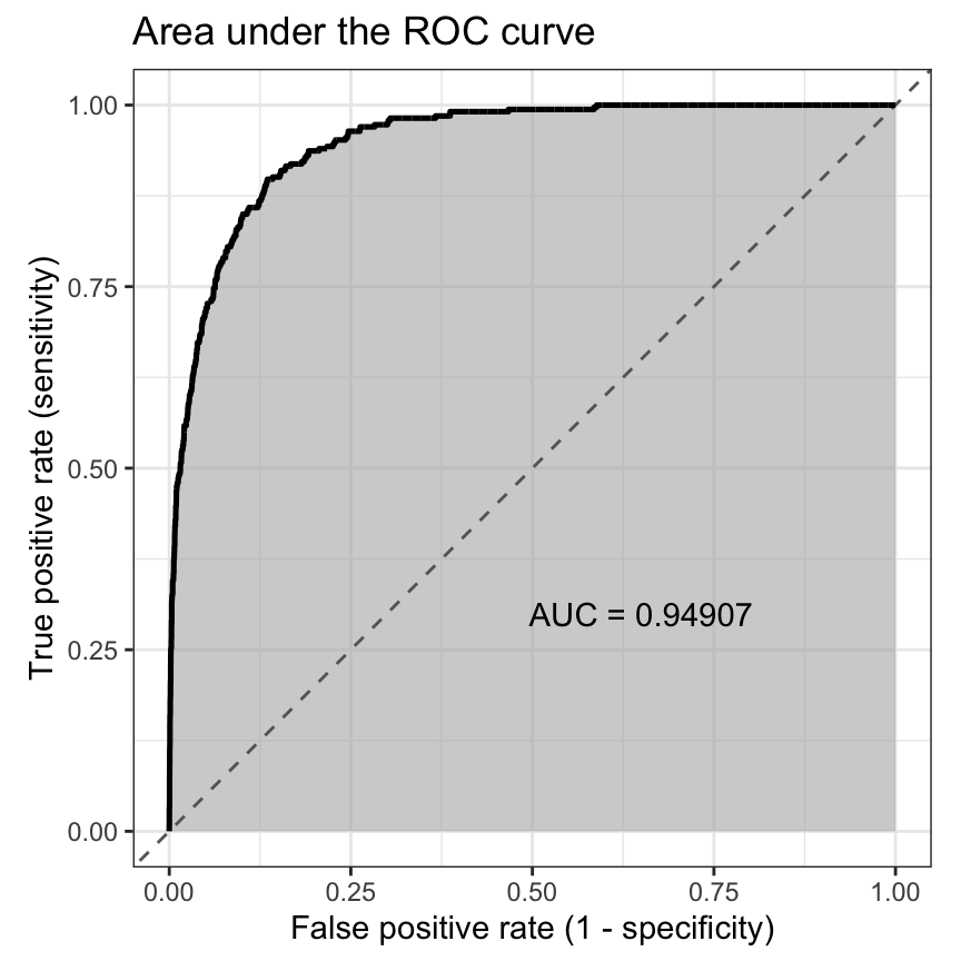
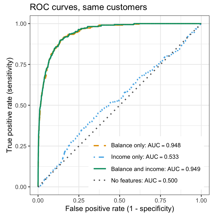
With balance alone, LDA and logistic regression have identical AUCs of 0.94798: both posterior probabilities are increasing functions of balance, so they order the customers identically and trace the same ROC curve. With balance and income, the two classifiers’ posterior probabilities weight income differently relative to balance, so their orderings differ slightly. Their AUCs, 0.94907 and 0.94905, differ by $2.1 \times 10^{-5}$. An AUC of 0.949, close to 1, reflects an ROC curve that bows far toward the top-left corner.

In the right panel, the AUC ranks the classifiers without a threshold. Income alone barely separates the classes: its curve stays near the diagonal, even dipping below it in places, and its AUC is 0.533. The balance-only and two-feature curves nearly coincide and cross: the two-feature curve is the higher one over 27% of the range of false positive rates and the balance-only curve over 11%. When two classifiers’ ROC curves cross, each has the higher true positive rate over part of the range of false positive rates, and the AUC averages the true positive rate over all false positive rates, so the classifier with the larger AUC can still be the worse one over the false positive rates that matter for a given application.

14.3 Credit card findings

LDA with balance and income identifies defaulters about as well as the logistic regression with the same features: although its Gaussian assumptions fit these customers imperfectly, it orders them almost exactly as logistic regression does, and differs mainly in flagging fewer customers at high thresholds. Income adds little to classification beyond balance, raising LDA’s AUC by 0.0011, although its logistic regression coefficient is clearly nonzero ($z = 4.17$). At $t = 0.5$ either classifier catches only a minority of defaulters, so a lender that cares about missed defaults would use a lower threshold.

14.4 Student strata

Student status has not entered any model so far. This additional analysis asks whether separate models for students and non-students classify better. The table below gives each stratum’s number of customers, number of defaulters, default rate, and median income.

Code

strata <- c(No = "No", Yes = "Yes")
in_stratum <- map(strata, \(s) filter(Default, student == s))
strata_summary <- Default |>
  group_by(student) |>
  summarize(n = n(), defaulters = sum(default == "Yes"),
            rate = mean(default == "Yes"), median_income = median(income),
            min_income = min(income), max_income = max(income),
            .groups = "drop")
strata_summary_of <- function(s, col) {
  strata_summary[[col]][strata_summary$student == s]
}
strata_summary_table <- strata_summary |>
  transmute(student, n = format(n, big.mark = ","), defaulters,
            rate = sprintf("%.2f%%", 100 * rate),
            median_income = paste0("\\$", dollars(median_income))) |>
  knitr::kable(col.names = c("Student", "Customers", "Defaulters",
                             "Default rate", "Median income"),
               align = "ccccc")

Student	Customers	Defaulters	Default rate	Median income
No	7,056	206	2.92%	$39,893
Yes	2,944	127	4.31%	$17,994

Students default more often than non-students, 4.31% against 2.92%, and, as the LDA lecture noted, their median income is far lower.

The figure below plots income against balance separately for non-students and students, with defaulters and non-defaulters distinguished by color and shape, and each panel’s income axis covering its own stratum’s incomes.

Code

strata_data_plot <- scatter_base +
  facet_wrap(~ student, labeller = label_both, scales = "free_y") +
  labs(title = "ISLR2::Default, income against balance by student status")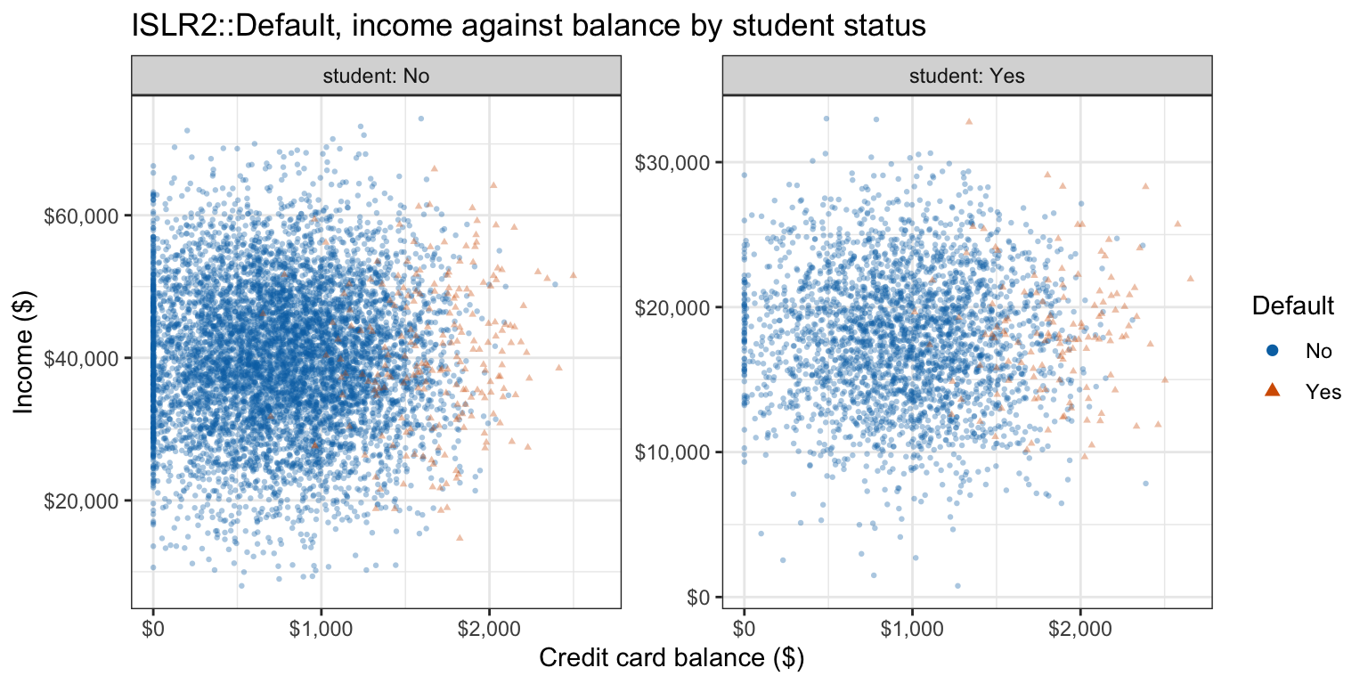

In both strata the defaulters sit at the larger balances. The students’ incomes occupy a lower, narrower band, from $772 to $33,003, against $8,018 to $73,554 for non-students.

Below, LDA with balance and income is fit separately to the non-students and the students, so its priors, class means, and pooled covariance can all differ by stratum. Beside it is the logistic regression in which the intercept and both slopes interact with student status. Each customer is scored by the model for its own stratum. Because each stratum’s priors are its own default rates, each posterior estimates the probability of default given balance, income, and student status, so posteriors from the two strata are on one scale and can be compared with each other.

Code

strata_lda <- map(in_stratum, \(d) MASS::lda(default ~ balance + income, data = d))
strata_glm <- map(in_stratum, \(d) glm(default ~ balance + income, data = d,
                                       family = "binomial"))
interacted_glm <- glm(default ~ (balance + income) * student, data = Default,
                      family = "binomial")

# Score every customer with its own stratum's model.
by_stratum <- function(score) {
  p <- numeric(nrow(Default))
  for (s in strata) p[Default$student == s] <- score(s)
  p
}
post_lda_strat <- by_stratum(\(s) {
  predict(strata_lda[[s]], newdata = in_stratum[[s]])$posterior[, "Yes"]
})
post_glm_strat <- by_stratum(\(s) fitted(strata_glm[[s]]))
max_diff_int <- max(abs(fitted(interacted_glm) - post_glm_strat))

strata_metrics <- imap(list(
  "LDA, single fit" = post_lda_2, "LDA, by student stratum" = post_lda_strat,
  "Logistic regression, additive" = post_glm_2,
  "Logistic regression, interacted with student" = fitted(interacted_glm)
), \(p, nm) {
  m <- metrics(confusion_counts(p, 0.5))
  tibble(model = nm, error = m[["error"]],
         auc = auc_trapezoid(roc_curve(p, is_yes)))
}) |>
  list_rbind()
strata_of <- function(m, col) strata_metrics[[col]][strata_metrics$model == m]
strata_table <- strata_metrics |>
  mutate(error = sprintf("%.4f", error), auc = sprintf("%.5f", auc)) |>
  knitr::kable(col.names = c("Model", "Error rate at $t = 0.5$", "AUC"),
               align = "lcc")

# Each stratum's boundary from each model, with its balance threshold at the
# stratum's median income.
strata_hand <- map(in_stratum, \(d) lda_by_hand(d[c("balance", "income")],
                                                 d$default))
strata_lines <- imap(strata, \(s, nm) {
  h <- strata_hand[[s]]
  b <- coef(strata_glm[[s]])
  tibble(student = s, model = c("LDA", "Logistic regression"),
         b0 = c(h$beta0, b[[1]]), b1 = c(h$beta[[1]], b[[2]]),
         b2 = c(h$beta[[2]], b[[3]]))
}) |>
  list_rbind() |>
  left_join(strata_summary |>
              transmute(student = as.character(student), median_income),
            by = "student") |>
  mutate(intercept = -b0 / b2, slope = -b1 / b2,
         threshold = threshold_at(b0, b1, b2, median_income))
strata_value <- function(s, col, m = "LDA") {
  strata_lines[[col]][strata_lines$student == s & strata_lines$model == m]
}
# The LDA and logistic boundaries of a stratum cross where their balance
# thresholds are equal. If each crossing lies outside the incomes the stratum
# has, and logistic regression's threshold is lower at the median income,
# logistic regression's boundary is left of LDA's throughout.
boundary_crossing <- function(s) {
  l <- filter(strata_lines, student == s)
  (l$b0[2] / l$b1[2] - l$b0[1] / l$b1[1]) /
    (l$b2[1] / l$b1[1] - l$b2[2] / l$b1[2])
}
glm_left_throughout <- all(map_lgl(strata, \(s) {
  cr <- boundary_crossing(s)
  inc <- in_stratum[[s]]$income
  (cr < min(inc) || cr > max(inc)) &&
    strata_value(s, "threshold", "Logistic regression") <
      strata_value(s, "threshold")
}))

# How much the students' larger prior alone lowers their LDA threshold:
# the change in log prior odds, converted to balance by the balance slope.
log_prior_odds <- function(h) log(h$pi[2] / h$pi[1])
prior_shift <- (log_prior_odds(strata_hand$Yes) - log_prior_odds(strata_hand$No)) /
  strata_hand$Yes$beta[[1]]
# Class mean balances by stratum, and the midpoint of each stratum's pair.
class_mean <- function(s, k) strata_hand[[s]]$mu[k, "balance"]
midpoint_shift <- mean(strata_hand$Yes$mu[, "balance"]) -
  mean(strata_hand$No$mu[, "balance"])
# Students' minus non-students' LDA threshold over the incomes both strata
# have; the thresholds are linear in income, so the ends bound the gap.
overlap <- c(max(strata_summary$min_income), min(strata_summary$max_income))
threshold_gap <- threshold_at(strata_hand$Yes$beta0, strata_hand$Yes$beta[[1]],
                              strata_hand$Yes$beta[[2]], overlap) -
  threshold_at(strata_hand$No$beta0, strata_hand$No$beta[[1]],
               strata_hand$No$beta[[2]], overlap)

# LDA estimates K - 1 priors, K p means, and p (p + 1) / 2 covariances.
K <- nlevels(Default$default)
p_features <- length(c("balance", "income"))
n_par_lda <- (K - 1) + K * p_features + p_features * (p_features + 1) / 2

strata_plot <- scatter_base +
  boundary_layers(strata_lines) +
  # Each panel's income axis covers its own stratum's incomes.
  facet_wrap(~ student, labeller = label_both, scales = "free_y") +
  labs(linetype = "Boundary",
       title = "Boundaries fit within each student stratum")

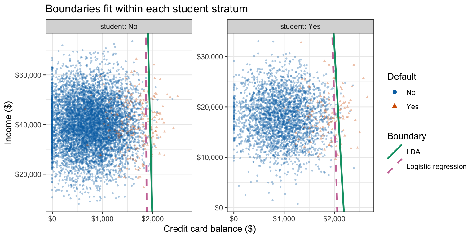
The table gives the training error rate at $t = 0.5$ and the AUC of these two models and of the single LDA and additive logistic regression of the earlier sections, all computed on the training customers. The figure repeats the scatterplot of income against balance for each stratum, over that stratum’s own range of income, with each stratum’s LDA boundary (solid green) and interacted logistic regression boundary (dashed pink).

Model	Error rate at $t = 0.5$	AUC
LDA, single fit	0.0276	0.94907
LDA, by student stratum	0.0273	0.94955
Logistic regression, additive	0.0263	0.94905
Logistic regression, interacted with student	0.0268	0.94958

Fitting the logistic regression with every coefficient interacted with student status is the same as fitting separate logistic regressions to the two strata: the two give the same fitted probabilities, to within $9 \times 10^{-15}$.

The extra flexibility barely changes the classifications. Stratifying LDA moves its training error rate from 2.76% to 2.73% and its AUC from 0.9491 to 0.9495; interacting the logistic regression with student status moves its error rate from 2.63% to 2.68% and its AUC from 0.9491 to 0.9496. The pooled ROC curve sweeps one threshold over the customers of both strata together, so it compares students’ scores with non-students’ as well as within each stratum. These are training rates, and the stratified models estimate twice as many parameters — 16 against 8 for LDA (1 prior, 4 means, and 3 covariance entries per fit), and 6 against 3 for logistic regression — so their training error rates tend to understate test error, and their training AUCs to overstate test AUC, by more; whether stratifying helps on new customers is a question for test data.

At each stratum’s median income, LDA’s balance threshold is $1,947 for non-students and $2,080 for students, and logistic regression’s is $1,869 and $2,005. Over the incomes each stratum actually has, logistic regression’s boundary lies to the left of LDA’s.

The students’ larger prior for Yes alone would lower their LDA threshold by $88. Their threshold is higher nonetheless because students in both classes carry higher balances: non-defaulting students average $948 against $745 for non-students, and defaulting students $1,860 against $1,678, which puts the midpoint of the students’ class means $193 higher. This is the confounding of the Multiple Logistic Regression lecture. Over the incomes both strata have, $8,018 to $33,003, the students’ threshold minus the non-students’ ranges from $38 to $152, so it stays higher when the strata are compared at the same income.

14.5 Conclusion

A classifier’s error rate hides which mistakes it makes. The confusion matrix separates them, sensitivity and specificity measure performance within each true class, and moving the threshold trades one against the other. With $K$ classes the confusion matrix is $K \times K$ and sensitivity and specificity are computed one class versus the rest. The ROC curve displays the two-class tradeoff at every threshold and depends only on how a classifier orders the observations. Its area, the AUC, is at most 1 with larger values generally better, is computed from the points of the ROC curve by the trapezoid rule, and ranks classifiers without fixing a threshold, although a classifier with the larger AUC can be the worse one over the false positive rates that matter for an application.

Fitting a model separately within each stratum of a categorical variable lets every parameter differ by stratum; for logistic regression it is the same as interacting every coefficient with that variable. Stratified models estimate more parameters, so their training error rates and training AUCs are more optimistic, and whether stratifying helps is a question for test data. When each stratum’s model uses that stratum’s own class proportions as priors, the posteriors from different strata share one scale, so a single error rate and AUC can be computed over all observations.

The next lecture returns to generative classifiers. Quadratic discriminant analysis relaxes LDA’s shared covariance matrix, giving each class its own, and naive Bayes replaces the multivariate Gaussian with a product of one-feature densities. That lecture then adds K-nearest neighbors and compares the classifiers on a held-out test set.

Truth	Predicted 1	Predicted 2	\(\cdots\)	Predicted \(K\)
1	\(n_{11}\)	\(n_{12}\)	\(\cdots\)	\(n_{1K}\)
2	\(n_{21}\)	\(n_{22}\)	\(\cdots\)	\(n_{2K}\)
\(\vdots\)	\(\vdots\)	\(\vdots\)	\(\ddots\)	\(\vdots\)
\(K\)	\(n_{K1}\)	\(n_{K2}\)	\(\cdots\)	\(n_{KK}\)